SRQ seminar – October 12th, 2018

Notes from a talk in the SRQ series.

INI Seminar 20181012 Toninelli

Interacting dimer models (lecture 3)

Partition function

$\displaystyle Z_{\Lambda, \lambda} = e^{W_{\Lambda, \lambda} (\underline{0})},$

$\displaystyle e^{W_{\Lambda, \lambda} (A)} = \sum_M \left[ \prod_{e \in M} t_e \right] e^{\lambda W (M) + \sum_e A_e \mathbb{I}_{e \in M}},$

where $A = \{ A_e \}_{e \in \text{edges of $\Lambda$}}$ is a source variable to generate the multi–edge correlations.

Grassmann representation

$\displaystyle e^{W_{\Lambda, \lambda = 0} (A)} = \int \mathrm{D} \psi e^{S_A (\psi)}, \qquad S_A (\psi) = - \sum_{\text{edges $e$}} E_e e^{A_e}$

with $E_e = \psi^+_x \psi^-_y \mathcal{K} (e)$ for an edge $e = (b_x, w_y)$.

Proposition 1. For the interaction

$\displaystyle W (M) = \sum_{\text{even faces $f$}} \left( \mathbb{I}_{\text{\scriptsize{$\begin{array}{l} \hline f\\ \hline \end{array}$}}} +\mathbb{I}_{\text{\scriptsize{$\begin{array}{|l|} f \end{array}$}}} \right)$

we have

$\displaystyle e^{W_{\Lambda, \lambda} (A)} = \int \mathrm{D} \psi e^{S_A (\psi) + \alpha \sum_{\gamma} \prod_{e \in \gamma} E_e e^{A_e}},$

where $\alpha = e^{\lambda} - 1$.

Proof. For simplicity let us fix $A = \underline{0}$.

$\displaystyle Z_{\Lambda, \lambda} = \sum_{\text{matchings $M$}} p (M) \underbrace{\prod_{\text{even $f$}} \left( 1 + \alpha \mathbb{I}_{\text{\scriptsize{$\begin{array}{|l|} f \end{array}$}}} \right) \left( 1 + \alpha \mathbb{I}_{\text{\scriptsize{$\begin{array}{l} \hline f\\ \hline \end{array}$}}} \right)}_{\prod_{\gamma = \{ e, e' \}} (1 + \alpha \mathbb{I}_{e \in M} \mathbb{I}_{e' \in M})}$

expanding the product we obtain

$\displaystyle = \sum_{\text{matchings $M$}} p (M) \sum_{n \geqslant 0} \sum_{\{ \gamma_1, \ldots, \gamma_n \}} \xi (\gamma_1) \cdots \xi (\gamma_n)$

where $\xi (\gamma) = \alpha \mathbb{I}_{e \in M} \mathbb{I}_{e' \in M}$ for $\gamma = \{ e, e' \}$. The various $\gamma$s do not shar edges even if they can share vertices (this do not cause problems). All these terms are of the type

$\displaystyle \sum_M p (M) \mathbb{I}_{e_1 \in M} \cdots \mathbb{I}_{e_{2 n} \in M} .$

These expressions can be obtained by the generating function as

$\displaystyle = \partial_{A_1} \ldots \partial_{A_n} e^{W_{\Lambda, \lambda = 0} (A)} |_{A = 0},$

and since we have already an expression for this we get

$\displaystyle = \int \mathrm{D} \psi e^{S_{A = 0} (\psi)} E_{e_1} \cdots E_{e_{2 n}},$

now we have just to resum to obtain the formula in the statement.$\Box$

Quasi–particle fields

A naive expansion of the partition functions in powers of $\alpha$ is divergent, so the point is to have a clever way to resum the naive expansion in a suitable way.

We are going to make a change of variables for the Grassmann fields introducing quasi–particle fields

$\displaystyle g (x, y) =\mathcal{E}_0 (\psi^-_x \psi^+_y) = \int \frac{\mathrm{d} p}{(2 \pi)^2} \frac{e^{i p \cdot (x - y)}}{\mu (p)} (\chi^+ (p) + \chi^- (p)) =: g_+ (x, y) + (- 1)^{x - y} g_- (x, y)$

where $\chi^{\pm}$ are functions concentrated near the singularities, $\chi^+$ around $(0, 0)$ and $\chi^-$ is around $(\pi, \pi)$ and they form a partition of unity: $\chi^+ (p) + \chi^- (p) = 1$. Then

$\displaystyle g_{\omega} (x, y) \approx \frac{1}{\phi_{\omega} (x, y)} \qquad \text{for $| x - y | \rightarrow \infty$}$

where $\phi_+ (x) = ((- i - 1) x_1 + (i + 1) x_2)$ and $\phi_- (x) = - \phi_+^{\ast} (x)$.

In terms of fields this splitting can be interpreted as $\psi^{\pm}_{x, \pm} = \psi^{\pm}_{x, +} + (- 1)^{(x_1 + x_2)} \psi^{\pm}_{x, -}$ and we use the addition principle for Grassmann variables. If $\mathcal{E}_g$ is an expectation for a field $\psi$ which satisfies the Wick rule for propagator $g$ and we split $g = g_1 + g_2$ then we can split $\psi = \psi_1 + \psi_2$ such that the first has propagator $g_1$, and $\psi_2$ with propagator $g_2$ and the mixed propagator is $0$.

$\displaystyle \mathcal{E}_g (f (\psi)) =\mathcal{E}_{\text{\scriptsize{$\left( \begin{array}{ll} g_1 & 0\\ 0 & g_2 \end{array} \right)$}}} (f (\psi_1 + \psi_2)) .$

This is analogous to the same property for Gaussians. You can verify the identity with $f (\psi)$ being a product of two.

Suppose we want to compute the partition function

$\displaystyle \log Z_{\Lambda, \lambda} = \log \int \mathrm{D} \psi e^{S (\psi) + \alpha V (\psi)},$

with $V (\psi) = \sum_{\gamma = (e, e')} E_e E_{e'}$ and $\psi = \{ \psi^+_x, \psi^-_x \}_{x \in \Lambda} = \{ \psi^+_{x, \omega}, \psi^-_{x, \omega} \}_{x \in \Lambda, \omega = \pm}$ and $\alpha = e^{\lambda - 1}$. By Taylor expansion (without worrying about convergence) one gets:

$\displaystyle \log \frac{Z_{\Lambda, \lambda}}{Z_{\Lambda, 0}} = \sum_{n \geqslant 1} \frac{1}{n!} \alpha^n \mathcal{E}_0 (\underbrace{V ; V ; \cdots ; V}_{\text{$n$ times}}),$

where

$\displaystyle \mathcal{E}_0 (\underbrace{V ; V ; \cdots ; V}_{\text{$n$ times}}) = \partial_{\lambda}^n \log \mathcal{E}_0 (e^{\lambda V}) |_{\lambda = 0} .$

Fact: $\mathcal{E}_0 (V ; \cdots ; V)$ is computed by performing contractions in Wick's rule for which all the blocks relating to different $V$'s form a connected set of blocks. (i.e. one consider the graph where edges are the Wick contractions and vertices are the set of fields belonging to the same $V$).

Remark 2. As long as the volume is finite all these expressions are well–defined and the expansion is convergent. Indeed at some point fields start repeating and they give zero. So the series is just a finite polynomial. And for $| \alpha | \ll 1$ one can take the log and everything is ok.

Remark 3. Single terms of this series can give problems as $\Lambda \rightarrow \infty$. Then there is the problem of the convergence of the series.

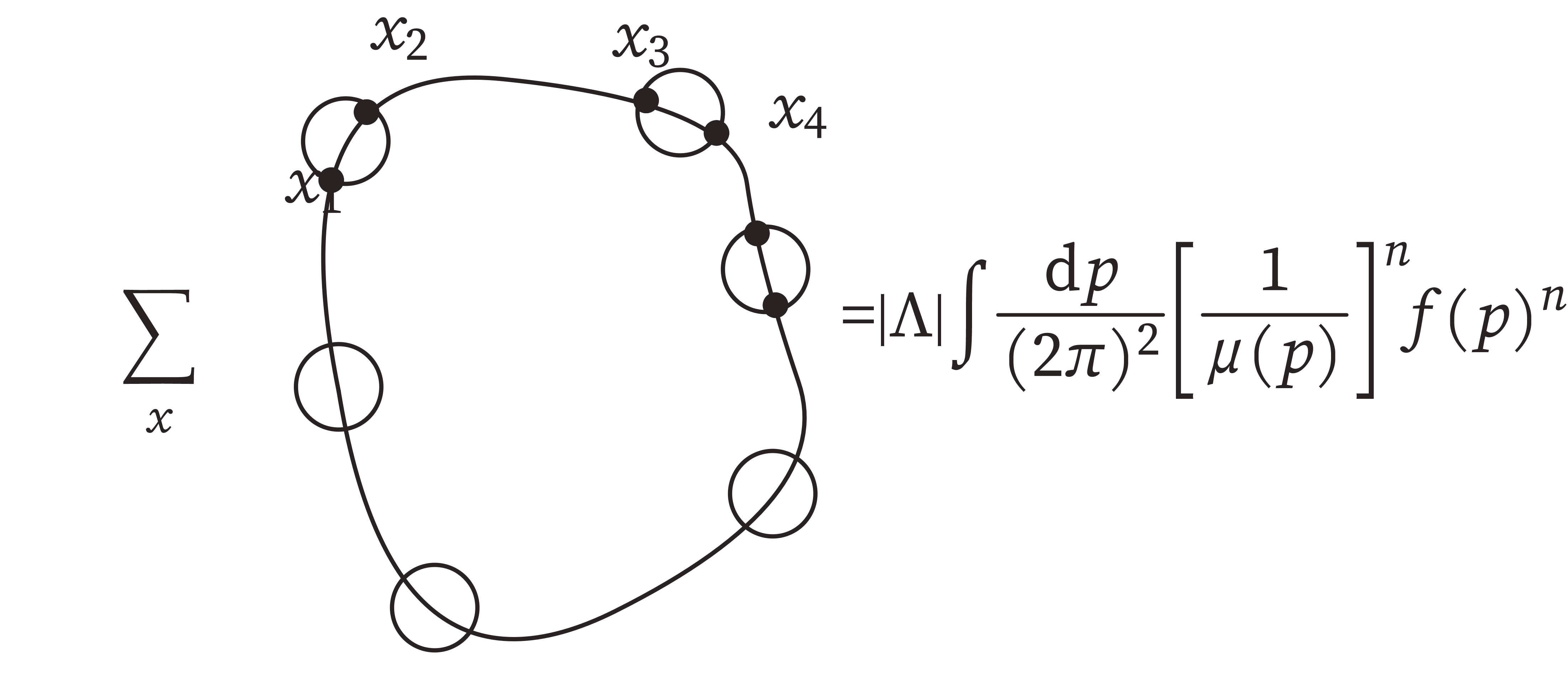
For graphs of the form

Figure from SRQ seminar – October 12th, 2018

and $f (p) \approx 1$ so there are singularities in the denominator as $n$ is not small. Here $f (p)$ is the contribution from the subgraph

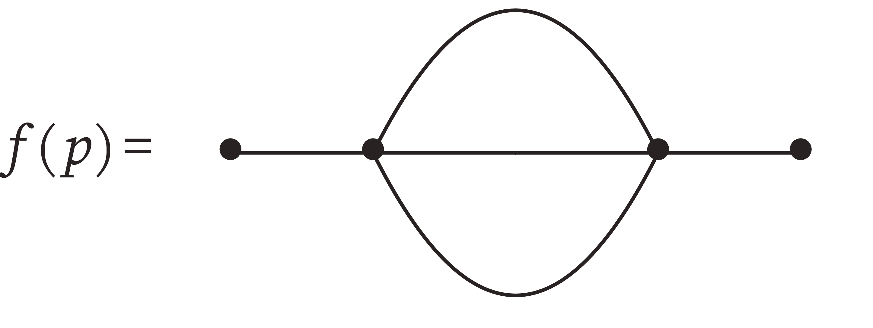
The idea is to break the propagator in dyadic pieces to localize the scale of the fluctuations and analyse better the behaviour near the singularity:

$\displaystyle g_+ (x) = \int \frac{\mathrm{d} p}{(2 \pi)^2} \frac{e^{i p \cdot x}}{\mu (p)} \chi_+ (p)$

Let $\chi_h (p) = \chi (2^{- h} p)$ and write

$\displaystyle \chi_+ (p) = \underbrace{\chi_+ (p) - \chi_{- 1} (p)}_{f_0 (p)} + \underbrace{\chi_{- 1} (p) - \chi_{- 2} (p)}_{f_1 (p)} + \underbrace{\chi_{- 2} (p) - \chi_{- 3} (p)}_{f_2 (p)} + \cdots + \chi_{h_L} (p)$

where $f_h$ is concentrated on disks where $| p | \approx 2^h$ and $h \leqslant 0$. $h_L = - \log_2 (L)$. We have now

$\displaystyle g_+ (x) = \sum_{h_L + 1}^0 g_+^{(h)} (x) + g_+^{(\leqslant h_L)} (x)$

and for fixed $h$ each $g_+^{(h)} (x)$ decay very fast since they are Fourier transforms of nice functions.

Proposition 4. For $h \leqslant 0$,

$\displaystyle | g_+^{(h)} (x) | \leqslant C 2^h e^{- \sqrt{2^h | x |}} .$

Multi–scale expansion

According to this decomposition of the propagator we have a multiscale expansion of the fermionic fields as:

$\displaystyle \psi^{\pm}_{x, \omega} = \sum_{h = h_L}^0 \psi^{\pm, (h)}_{x, \omega} .$

$\displaystyle Z =\mathcal{E} (e^{\alpha V (\psi)}) =\mathcal{E} (e^{\alpha V (\psi^{(0)} + \psi^{(- 1)} + \psi^{(- 2)} + \cdots)}) =\mathcal{E}_{h_L} \cdots \mathcal{E}_0 \left( e^{\alpha V (\psi^{(0)} + \psi^{(- 1)} + \psi^{(- 2)} + \cdots + \psi^{(h_L)})} \right)$

so we start by integrating out the scale $\psi^{(0)}$ and going forward. If we let $V^{(0)} = V$ and recursively $V^{(- 1)}$ as the result of the integration

$\displaystyle e^{\alpha V^{(- 1)} (\psi^{(- 1)} + \psi^{(- 2)} + \cdots + \psi^{(h_L)})} := \mathcal{E}_0 \left( e^{\alpha V (\psi^{(0)} + \psi^{(- 1)} + \psi^{(- 2)} + \cdots + \psi^{(h_L)})} \right)$

obtaining the formula

$\displaystyle V^{(- 1)} (\psi^{(\leqslant - 1)}) = \sum_n \frac{\alpha^n}{n!} \mathcal{E}_0 (V^{(0)} (\psi^{(0)} + \psi^{(\leqslant - 1)}) ; \cdots ; V^{(0)} (\psi^{(0)} + \psi^{(\leqslant - 1)})) .$

Going on to expand and introducing proper notations to label the results of the integrations as polynomials in the remaning variables one obtains:

$\displaystyle V^{(- 1)} (\psi^{(\leqslant - 1)}) = \sum_{n \geqslant 1} \frac{\alpha^n}{n!} \sum_{\tau \in \mathcal{T}^{(- 1)}_n} \sum_{P_{v_0} = \varnothing} \mathcal{E}_0 (\psi^{(0)} (P_{v_1}) ; \cdots ; \psi^{(0)} (P_{v_n}))$

$\displaystyle + \sum_{n \geqslant 1} \frac{\alpha^n}{n!} \sum_{\tau \in \mathcal{T}^{(- 1)}_n} \sum_{P_{v_0} \neq \varnothing} \mathcal{E}_0 (\psi^{(0)} (P_{v_1} \backslash Q_{v_1}) ; \cdots ; \psi^{(0)} (P_{v_n} \backslash Q_{v_n})) [\psi^{(\leqslant - 1)} (Q_{v_1}) \cdots \psi^{(\leqslant - 1)} (Q_{v_n})]$

$P_{v_k}$ is the collection of indexes of the fields appearing in the $k$-the leaf of the vertex $v$...

[but this part I didn't managed to follow...]