|
Abstract
We decompose the Gaussian free field along a scale parameter and take as primary objects the stochastic observables: martingales in the filtration of finite-resolution measurements. Interactions are introduced through the Polchinski equation for the effective potential. Its probabilistic counterpart is a forward–backward stochastic differential equation (FBSDE) for the field seen at increasing resolution, whose effective force is a martingale. Writing the FBSDE in the coordinate given by the conditional mean of the terminal field removes its drift and integrates the transport part of the force flow exactly. In the gradient case the remaining equation for the force is the Wetterich equation for the effective average action, whose propagator is the conditional covariance. We then discuss the variational structure of the flow (Boué–Dupuis formula and Hamilton–Jacobi–Bellman equation) in finite and infinite volume. The additional material covers Wick powers as observables in every dimension and their products (operator product expansion), the algebraic and perturbative structure of the flow (semigroup, flatness, counterterms for \(\Phi^4_3\)), and the Dyson–Schwinger equations at every scale. The treatment is formal: we compute as if all objects were smooth and integrable, and we indicate where the real difficulties lie.
Introduction 2
Structure. 3
What is formal. 3
Conventions. 3
Part I. Main lecture 3
4Setting: covariance profiles and observables 3
4.1Covariance profiles 3
4.2Stochastic observables 4
Exercises 5
5Interactions: the Polchinski equation and FBSDEs 5
5.1Effective potentials 5
5.2The Polchinski process 6
5.3Observables of the interacting theory 8
Tangent observables. 8
5.4The force and a Burgers equation 8
Exercises 9
6The FBSDE in force coordinates: the Wetterich equation 9
6.1State and costate 9
6.2Removing the predictable drift 9
6.3The FBSDE in the forecast coordinate 10
6.4Conditional moments 11
6.5The gradient sector: Wetterich's equation 11
6.6Variational meaning and the tree level 13
Constrained free energies. 13
The tree level. 13
Exercises 14
7Variational structure 14
7.1Finite volume: the Boué–Dupuis formula 14
Euler–Lagrange equation \(=\) FBSDE. 15
Entropy. 15
Generating functionals. 15
7.2Infinite volume 15
Exercises 16
Part II. Additional material 16
8Observables of the Gaussian free field and their products 16
8.1Wick powers and exponentials 16
Point evaluations. 16
Wick powers. 16
Exponentials. 16
8.2Products of observables 17
Products of point evaluations. 17
Operator product expansion. 17
Locality and factorisation. 17
Exercises 18
9Algebraic structure of the Polchinski flow 18
9.1A semigroup of renormalisation maps 18
9.2Perturbation theory and counterterms 19
Exercises 20
10Dyson–Schwinger equations at every scale 20
Exercises 21
References 21
In Lectures 1–2 a Euclidean field was a probability measure on \(\mathcal{S}' (\mathcal{M})\), i.e. a random distribution \(\varphi\), and local operators were functions of \(\varphi\). This viewpoint hides the scale-by-scale organisation of the Wilson–Kadanoff picture [WK74], and forces us to work with singular objects from the start. Already for the GFF, the Wick power \(: \varphi^n\): is not a random distribution when \(n (d - 2) \geq d\), since its regularisations are not even tight (Proposition 3.11 of Lecture 2).
In this lecture we index everything by a resolution \(t \in [0, \infty)\). The field observed at resolution \(t\) is a smooth function \(\varphi_t\), and the information available at resolution \(t\) is the \(\sigma\)-algebra \(\mathcal{F}_t\) generated by \((\varphi_s)_{s \leq t}\). A physical quantity is then not a single random variable but a consistent family of finite-resolution estimates of it, i.e. a martingale. This is the notion of stochastic observable of [BCG26], on which this lecture is based; see also [Pol84, BK87, Sal99, BBD24] for the renormalisation group side and [BG20, BG24] for the variational side.
Definition
Our standard example is the heat profile
| \(\displaystyle Q_t := C \hspace{0.17em} \mathrm{e}^{- A / t^2}, \qquad \dot{Q}_t = \frac{2}{t^3} \hspace{0.17em} \mathrm{e}^{- A / t^2},\) | (4.1) |
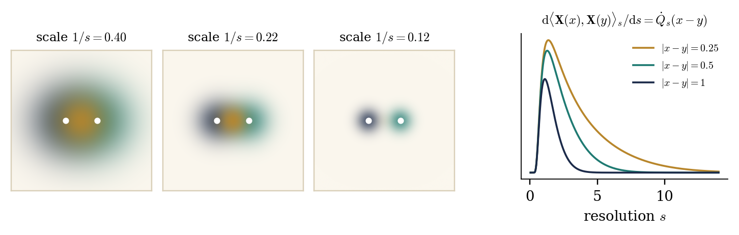
which smooths the Green function with the heat kernel at time \(t^{- 2}\). On \(\mathbb{R}^d\) the kernels are explicit,
| \(\displaystyle \dot{Q}_t (x - y) = \frac{2 t^{d - 3} \mathrm{e}^{- m^2 / t^2}}{(4 \pi)^{d / 2}} \hspace{0.17em} \mathrm{e}^{- t^2 |x - y|^2 / 4},\) | (4.2) |
so \(\dot{Q}_t\) is concentrated on distances \(\lesssim 1 / t\), and in Fourier space \(Q_t\) retains the modes \(|k| \lesssim t\): \(t\) is a momentum scale, or resolution. Other profiles are useful, even when they violate some smoothness requirement of Definition 4.1. A sharp Fourier cutoff is \(\hat{Q}_t (k) = \mathbb{1}_{|k| \leq t} (|k|^2 + m^2)^{- 1}\), which is not smooth in \(t\). In a finite range decomposition, \(\dot{Q}_t (x, y) = 0\) for \(|x - y| \geq 1 / t\) (Remark 8.4). We write
For \(d \geq 2\), \(c_t \to \infty\) as \(t \to \infty\) (Exercise 4.2).
Let \((W_t)_{t \geq 0}\) be a cylindrical Brownian motion on \(L^2 (\mathcal{M})\), \(\mathbb{E} [W_t (x) W_s (y)] = (t \wedge s) \delta (x - y)\), and
| \(\displaystyle X_t := \int_0^t \dot{Q}_s^{1 / 2} \hspace{0.17em} \mathrm{d} W_s .\) | (4.3) |
Proposition
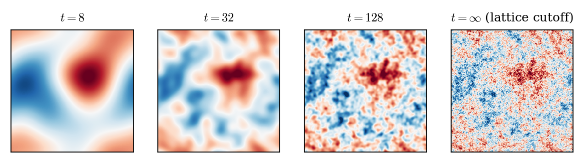
So the GFF is the terminal value of a Gaussian martingale of smooth fields: the field at resolution \(t\) (Figure 4.1). The proof is a variant of Theorem 3.2 of Lecture 2 and is left as Exercise 4.1.
Fix a filtration \((\mathcal{F}_t)_{t \geq 0}\), for the moment that of \(X\), and write \(\mathbb{E}_t := \mathbb{E}[\hspace{0.17em} \cdot \hspace{0.17em} |\mathcal{F}_t]\).
Definition
Every integrable \(\mathcal{F}_{\infty}\)-measurable random variable \(Y\) gives a closed observable \(O_t =\mathbb{E}_t [Y]\), with \(O_t \to Y\). The point of the definition is that interesting observables need not be closed: a martingale may diverge as \(t \to \infty\) (for instance \(X_t (x)\) for \(d \geq 2\)), and still carry a perfectly meaningful family of finite-resolution estimates. The next lemma is elementary but basic.
Lemma
Proof. (a) \(O^1_s - O^2_s =\mathbb{E}_s [O^1_t - O^2_t]\) for every \(t \geq s\), and conditional expectation is an \(L^1\) contraction. (b) Likewise, \(\|O_s -\mathbb{E}_s N_t \|_{L^1} \leq \|O_t - N_t \|_{L^1}\).\(\Box\)
So an observable is determined by its asymptotic behaviour. A germ for \(O\) is a family of functionals \(\ring{O}_t\) on smooth fields such that \(\|O_t - \ring{O}_t (X_t)\|_{L^1} \to 0\). The observable field \(O (x)\) is local if it admits germs of the form
Germs are not unique, and this freedom reflects the freedom of choosing counterterms. By Lemma 4.4(b), a germ determines the observable.
Exercise
Exercise
Fix a finite volume \(\mathcal{M}=\mathbb{T}^d_L\) and a terminal resolution \(T < \infty\), which plays the role of an ultraviolet cutoff: the reference field \(X_T \sim \mu^{Q_T}\) is smooth. Let \(V_T\) be an interaction, a functional of smooth fields bounded below. Our main example is
| \(\displaystyle V_T (\varphi) = \int_{\mathbb{T}^d_L} \left[ \lambda H_4 (\varphi (x) ; c_T) + \gamma_T \hspace{0.17em} H_2 (\varphi (x) ; c_T) \right] \mathrm{d} x,\) | (5.1) |
with a mass counterterm \(\gamma_T\) to be fixed in Section 9.2 (\(\gamma_T = 0\) for \(d = 2\)). The interacting measure at cutoff \(T\) is
| \(\displaystyle \nu_T (\mathrm{d} \varphi) = Z_T^{- 1} \mathrm{e}^{- V_T (\varphi)} \mu^{Q_T} (\mathrm{d} \varphi) .\) | (5.2) |
Definition
| \(\displaystyle \mathrm{e}^{- V_t (\varphi)} := \int \mathrm{e}^{- V_T (\varphi + \zeta)} \hspace{0.17em} \mu^{Q_{T, t}} (\mathrm{d} \zeta) .\) | (5.3) |
\(V_t\) is the interaction felt by the field at resolution \(t\) once the fluctuations between \(t\) and \(T\) have been integrated out: it is the Wilson effective action. At \(t = 0\), \(V_0 (0) = - \log Z_T\) is the free energy. Here is the first key fact.
Proposition
| \(\displaystyle \text{Law}_{\mathbb{P}} (X_t) = \nu_t, \qquad \nu_t (\mathrm{d} \varphi) := Z_T^{- 1} \mathrm{e}^{- V_t (\varphi)} \mu^{Q_t} (\mathrm{d} \varphi) .\) | (5.4) |
Moreover, the conditional law of \(X_T\) given \(\mathcal{F}_t\) is
| \(\displaystyle \mu_t^{X_t} (\mathrm{d} \varphi), \qquad \mu_t^{\phi} (G) := \mathrm{e}^{V_t (\phi)} \int G (\phi + \zeta) \hspace{0.17em} \mathrm{e}^{- V_T (\phi + \zeta)} \hspace{0.17em} \mu^{Q_{T, t}} (\mathrm{d} \zeta) .\) | (5.5) |
Proof. Under \(\mathbb{P}_0\), \(X_T = X_t + (X_T - X_t)\) with an independent increment of law \(\mu^{Q_{T, t}}\). Hence \(\mathbb{E}_{\mathbb{P}} [G (X_t)] = Z_T^{- 1} \mathbb{E}_0 [G (X_t) \mathrm{e}^{- V_T (X_T)}] = Z_T^{- 1} \mathbb{E}_0 [G (X_t) \mathrm{e}^{- V_t (X_t)}]\). The conditional law follows in the same way.\(\Box\)
So at every resolution the field is again a Gibbs measure, with reference covariance \(Q_t\) and potential \(V_t\). The measure-valued martingale \((\mu_t^{X_t})_t\) goes from \(\nu_T\) at \(t = 0\) to \(\delta_{X_T}\) at \(t = T\): it is a stochastic localisation of \(\nu_T\) in the sense of Eldan [Eld23], adapted to the covariance profile [BBD24, BCG26].
Theorem
| \(\displaystyle \partial_t V_t = \tfrac{1}{2} \langle DV_t, \dot{Q}_t \hspace{0.17em} DV_t \rangle - \tfrac{1}{2} \text{Tr} \left( \dot{Q}_t \hspace{0.17em} D^2 V_t \right), \qquad t \in [0, T],\) | (5.6) |
with terminal condition \(V_T\).
Proof. \(u_t := \mathrm{e}^{- V_t} = \mathrm{e}^{\frac{1}{2} \Delta_{Q_{T, t}}} u_T\) is a Gaussian convolution, where \(\Delta_Q := \text{Tr} (QD^2)\). Since \(\partial_t Q_{T, t} = - \dot{Q}_t\), it solves the backward heat equation \(\partial_t u_t = - \frac{1}{2} \text{Tr} (\dot{Q}_t D^2 u_t)\). Insert \(D^2 u = (DV \otimes DV - D^2 V) u\) and divide by \(- u\).\(\Box\)
The nonlinear term generates new, generally nonlocal, interactions (trees), and the trace term contracts pairs of fields with the covariance of the shell \([t, t + \mathrm{d} t]\) (loops). The substitution \(u = \mathrm{e}^{- V}\), which linearises the equation, is a Cole–Hopf transform: we come back to this in Section 5.4, and in Section 9.
Theorem
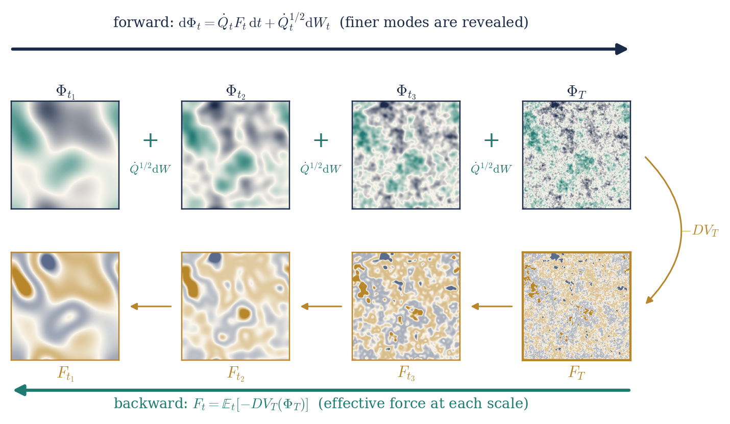
| \(\displaystyle \mathrm{d} \Phi_t = \dot{Q}_t \hspace{0.17em} F_t \hspace{0.17em} \mathrm{d} t + \dot{Q}_t^{1 / 2} \hspace{0.17em} \mathrm{d} W^{\mathbb{P}}_t, \qquad F_t = - DV_t (\Phi_t) =\mathbb{E}^{\mathbb{P}}_t [- DV_T (\Phi_T)],\) | (5.7) |
with \(\Phi_0 = 0\) and a \(\mathbb{P}\)-cylindrical Brownian motion \(W^{\mathbb{P}}\). In particular the effective force \((F_t)_{t \leq T}\) is a \(\mathbb{P}\)-martingale: an observable field of the interacting theory.
Proof. The density process is \(M_t := \mathbb{E}_0
[\mathrm{d} \mathbb{P}/ \mathrm{d} \mathbb{P}_0
|\mathcal{F}_t] = Z_T^{-
1} \mathrm{e}^{- V_t (X_t)}\), by Proposition 5.2. By
Itô's formula and
Read as an equation for an unknown pair \((\Phi, F)\),
| \(\displaystyle \Phi_t = \int_0^t \dot{Q}_s F_s \hspace{0.17em} \mathrm{d} s + \int_0^t \dot{Q}_s^{1 / 2} \mathrm{d} W_s, \qquad F_t =\mathbb{E}_t [- DV_T (\Phi_T)], \qquad t \in [0, T] .\) | (5.8) |
Here and below we drop the superscript and write \(W\) for the Brownian
motion driving the interacting field. The Polchinski equation is not
needed to state
|
Figure 5.1. The forward–backward
structure of |
Remark
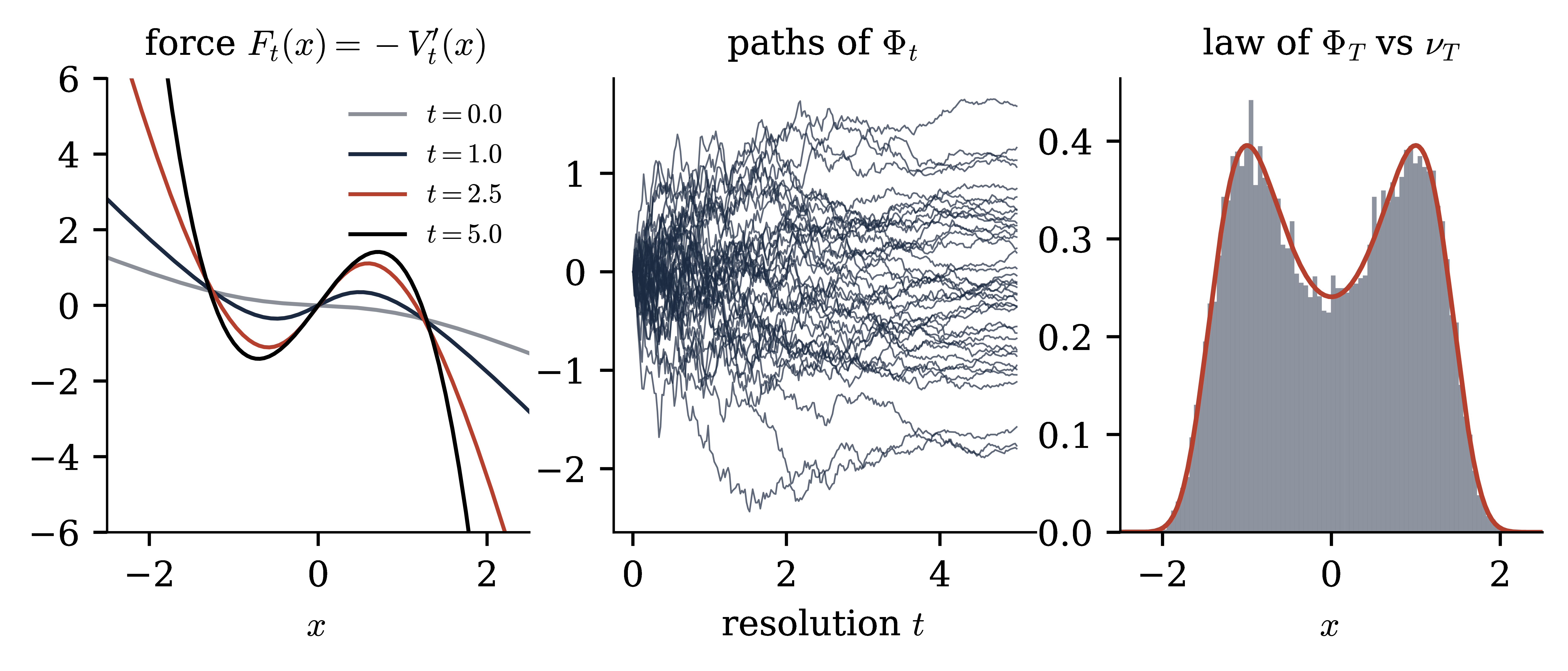
|
Figure 5.2. A zero-dimensional Polchinski
process (Exercise 5.2): \(Q_t = 1 - \mathrm{e}^{-
t}\), \(T = 5\), \(V_T (x) = \frac{1}{2} x^4 - \frac{3}{2}
x^2\). Left: the effective force \(F_t = - V_t'\) is almost
linear at low resolution and develops the double-well structure
as \(t \to T\). Centre: paths of the FBSDE |
For a functional \(G\) of the terminal field, the observable \(O_t =\mathbb{E}^{\mathbb{P}}_t [G (\Phi_T)]\) is \(O_t = G_t (\Phi_t)\), with
| \(\displaystyle G_t (\phi) = \mu_t^{\phi} (G) = \mathrm{e}^{V_t (\phi)} \int G (\phi + \zeta) \hspace{0.17em} \mathrm{e}^{- V_T (\phi + \zeta)} \mu^{Q_{T, t}} (\mathrm{d} \zeta) .\) | (5.9) |
Formally, \(G_t\) solves the backward Kolmogorov equation of the interacting dynamics,
| \(\displaystyle \partial_t G_t + \tfrac{1}{2} \text{Tr} (\dot{Q}_t D^2 G_t) - \langle \dot{Q}_t DV_t, DG_t \rangle = 0, \qquad G_T = G,\) | (5.10) |
which is the Doob transform of the Gaussian heat equation by
\(\mathrm{e}^{- V_t}\) (Exercise 5.3). Conversely, any
solution of
| \(\displaystyle \partial_{\theta} \mathbb{E}^{\nu^{\theta}_T} [G] = - \text{Cov}^{\nu_T^{\theta}} (G, \partial_{\theta} V^{\theta}_T) .\) | (5.11) |
Thus the tangent observables, such as the running \(: \varphi^4\): for \(\theta = \lambda\) (together with the derivative of the counterterm \(\partial_{\lambda} \gamma_T \int : \varphi^2\):), describe the response of the theory to a change of coupling. They are the observables conjugate to the coordinates of theory space.
Differentiating
| \(\displaystyle \partial_t F_t = - DF_t [\dot{Q}_t F_t] - \tfrac{1}{2} \text{Tr} (\dot{Q}_t D^2 F_t), \qquad F_T = - DV_T,\) | (5.12) |
an infinite-dimensional, backward, viscous Burgers equation.
The Cole–Hopf transform \(F = D \log u\) linearises it, which is
the statement that \(u = \mathrm{e}^{- V}\) solves a heat equation. Two
remarks on
it uses only the force, which is a local quantity (intensive), while \(V_t\) is extensive, of order of the volume. This matters in infinite volume (Section 7.2);
the Burgers flows for different covariances commute, and the curvature vanishes, when \(DF_t\) is symmetric, i.e. when \(F_t\) is a gradient [BCG26]. For a non-gradient force, as for the general Wilson–Itô diffusions of [BCG26], the flows do not commute.
Exercise
Exercise
Exercise
In this section the forward–backward system
is the covariance still unresolved at resolution \(t\), and \((\Phi,
F)\) solves
The FBSDE is the stochastic Pontryagin system of the control problem of Theorem 7.1. The controlled field \(\mathrm{d} X = \dot{Q}_t^{1 / 2} (u \hspace{0.17em} \mathrm{d} t + \mathrm{d} W)\) has Hamiltonian \(\langle p, \dot{Q}_t^{1 / 2} u \rangle - \frac{1}{2} \|u\|^2\), which does not depend on the state. By the stochastic maximum principle (Exercise 6.1), the adjoint process \(p\) has no drift, \(\mathrm{d} p_t = \Upsilon_t \hspace{0.17em} \mathrm{d} W_t\), with terminal value \(p_T = - DV_T (X_T)\), and the optimal control is \(u_t = \dot{Q}_t^{1 / 2} p_t\). Thus
the field \(\Phi\) is the state, and the force \(F\) is the costate.
The function \(F_t (\cdot)\) with \(F_t = F_t (\Phi_t)\) is the
decoupling field of the FBSDE, and the Burgers equation
Without noise the state–costate pair follows the Hamiltonian flow of the free Hamiltonian \(h_s (p) = \frac{1}{2} \langle p, \dot{Q}_s p \rangle\): \(\dot{p} = 0\) and \(\dot{x} = \dot{Q}_s p\). From \(t\) to \(T\) this flow is the linear shear
| \(\displaystyle \Sigma_t : (x, p) \longmapsto (x + S_t p, \hspace{0.27em} p) .\) | (6.1) |
Its trajectories are the characteristics of the transport part of
The drift \(\dot{Q}_t F_t\) of the state is predictable, and the costate
is a martingale. Hence the drift that remains to be accumulated on \([t,
T]\) is predicted, at resolution \(t\), by transporting the current
state with the current costate along the free flow
Proposition
| \(\displaystyle \psi_t := \mathbb{E}_t [\Phi_T] = \Phi_t + S_t F_t,\) | (6.2) |
i.e. \((\psi_t, F_t) = \Sigma_t (\Phi_t, F_t)\). It is a martingale, with
| \(\displaystyle \mathrm{d} \psi_t = \dot{Q}_t^{1 / 2} \mathrm{d} W_t + S_t \Upsilon_t \hspace{0.17em} \mathrm{d} W_t = (\mathbb{1} + S_t DF_t (\Phi_t)) \dot{Q}_t^{1 / 2} \mathrm{d} W_t .\) | (6.3) |
Proof. Integrate the forward equation from \(t\) to \(T\) and condition on \(\mathcal{F}_t\): since \(F\) is a martingale, \(\mathbb{E}_t \int_t^T \dot{Q}_s F_s \mathrm{d} s = S_t F_t\). For the differential, the drift \(\dot{Q}_t F_t\) of \(\Phi\) cancels against \(\dot{S}_t F_t\), and \(S_t \hspace{0.17em} \mathrm{d} F_t = S_t \Upsilon_t \hspace{0.17em} \mathrm{d} W_t\).\(\Box\)
So \(\psi\) is a closed observable, the field observable of [BCG26]. The field splits as
| \(\displaystyle \Phi_t = \psi_t - S_t F_t :\) | (6.4) |
a martingale, minus the drift still expected on the unresolved scales,
which vanishes at \(t = T\). The noise of \(\psi\) in
Assume that the map \(x \mapsto \psi = x + S_t F_t (x)\) is invertible, and write its inverse as
| \(\displaystyle x = \psi + S_t \mathscr{F}_t (\psi), \qquad \mathscr{F}_t (\psi) := - F_t (x),\) | (6.5) |
so that \(F_t = - \mathscr{F}_t (\psi_t)\): the costate is now a function of the forecast. Introduce the response and the regulator
| \(\displaystyle H_t (\psi) := (S_t^{- 1} + D \mathscr{F}_t (\psi))^{- 1}, \qquad \mathscr{R}_t := S_t^{- 1} - Q_T^{- 1}, \qquad \dot{\mathscr{R}}_t = S_t^{- 1} \dot{Q}_t S_t^{- 1} \geq 0.\) | (6.6) |
Differentiating the two maps \(x \leftrightarrow \psi\) gives \(\mathbb{1} + S_t DF_t (x) = (\mathbb{1} + S_t D \mathscr{F}_t (\psi))^{- 1} = H_t (\psi) S_t^{- 1}\).
Theorem
| \(\displaystyle \mathrm{d} \psi_t = H_t (\psi_t) \hspace{0.17em} S_t^{- 1} \dot{Q}_t^{1 / 2} \hspace{0.17em} \mathrm{d} W_t, \qquad \mathscr{F}_t (\psi_t) =\mathbb{E}_t [DV_T (\psi_T)],\) | (6.7) |
with \(\psi_0 = S_0 F_0 =\mathbb{E} [\Phi_T]\) and \(\psi_T = \Phi_T\). The forward equation has no drift, and its covariance is \(\mathcal{C}_t := H_t \dot{\mathscr{R}}_t H_t^{\ast}\). The decoupling field \(\mathscr{F}\) solves the pure diffusion equation
| \(\displaystyle \partial_t \mathscr{F}_t + \tfrac{1}{2} \hspace{0.17em} \text{Tr} \left( \mathcal{C}_t \hspace{0.17em} D^2 \mathscr{F}_t \right) = 0, \qquad \mathscr{F}_T = DV_T .\) | (6.8) |
Proof. The forward equation is
The backward equation is \(F_t =\mathbb{E}_t [F_T]\) with \(\psi_T =
\Phi_T\). Since \(\mathscr{F}_t (\psi_t)\) is a martingale and \(\psi\)
has no drift, the drift in Itô's formula for \(\mathscr{F}_t
(\psi_t)\) is the left-hand side of
Compare
For the Polchinski process the response has a direct meaning.
Proposition
In particular \(H_t > 0\) is symmetric, \(\mathbb{1} + S_t DF_t = \text{Cov}_t S_t^{- 1}\) is always invertible, and \(H_t \leq S_t\) when \(V_T\) is convex.
Proof. By
So the forecast coordinates are the first two conditional moments of the stochastic localisation \(\mu_t^{\Phi_t}\) of Proposition 5.2: \((\psi_t, \text{Cov}_t) = (\mathbb{E}_t \Phi_T, \text{Cov}_t \Phi_T)\) (Figure 6.1). They are tied by Itô's formula: since \(\mathbb{E}_t [\Phi_T \otimes \Phi_T] = \psi_t \otimes \psi_t + \text{Cov}_t\) is a martingale,
| \(\displaystyle \mathrm{d} \langle \psi, \psi \rangle_t =\mathcal{C}_t \hspace{0.17em} \mathrm{d} t = \text{Cov}_t \dot{\mathscr{R}}_t \text{Cov}_t \hspace{0.17em} \mathrm{d} t, \qquad \text{dCov}_t = - \text{Cov}_t \dot{\mathscr{R}}_t \text{Cov}_t \hspace{0.17em} \mathrm{d} t + \mathrm{d} (\text{martingale}) .\) | (6.9) |
Conditional variance is resolved at the rate \(\text{Cov}_t \dot{\mathscr{R}}_t \text{Cov}_t\), which for the Gaussian reference is \(S_t \dot{\mathscr{R}}_t S_t = \dot{Q}_t\).
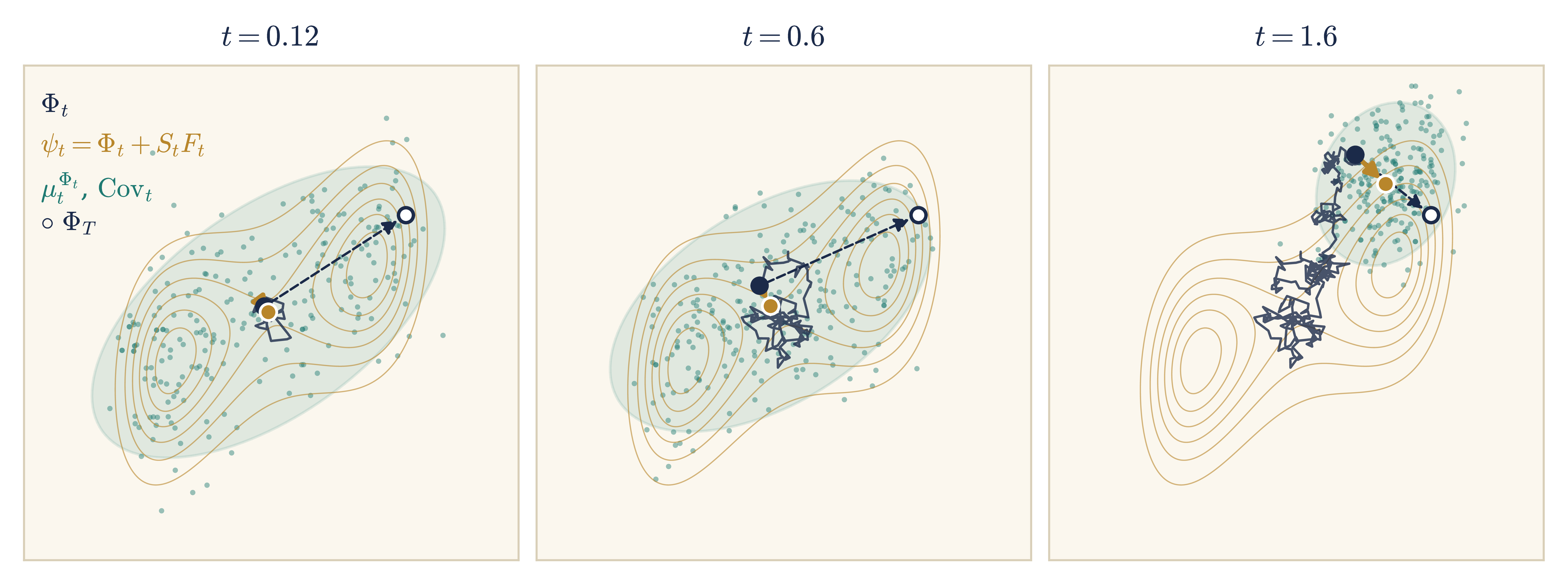
|
Figure 6.1. Stochastic localisation for a
two-component field: \(Q_t = (1 - \mathrm{e}^{- t})
\mathbb{1}\), \(T = 4\), \(V_T\) a tilted double well, and the
contours show the density of \(\nu_T\). One path of |
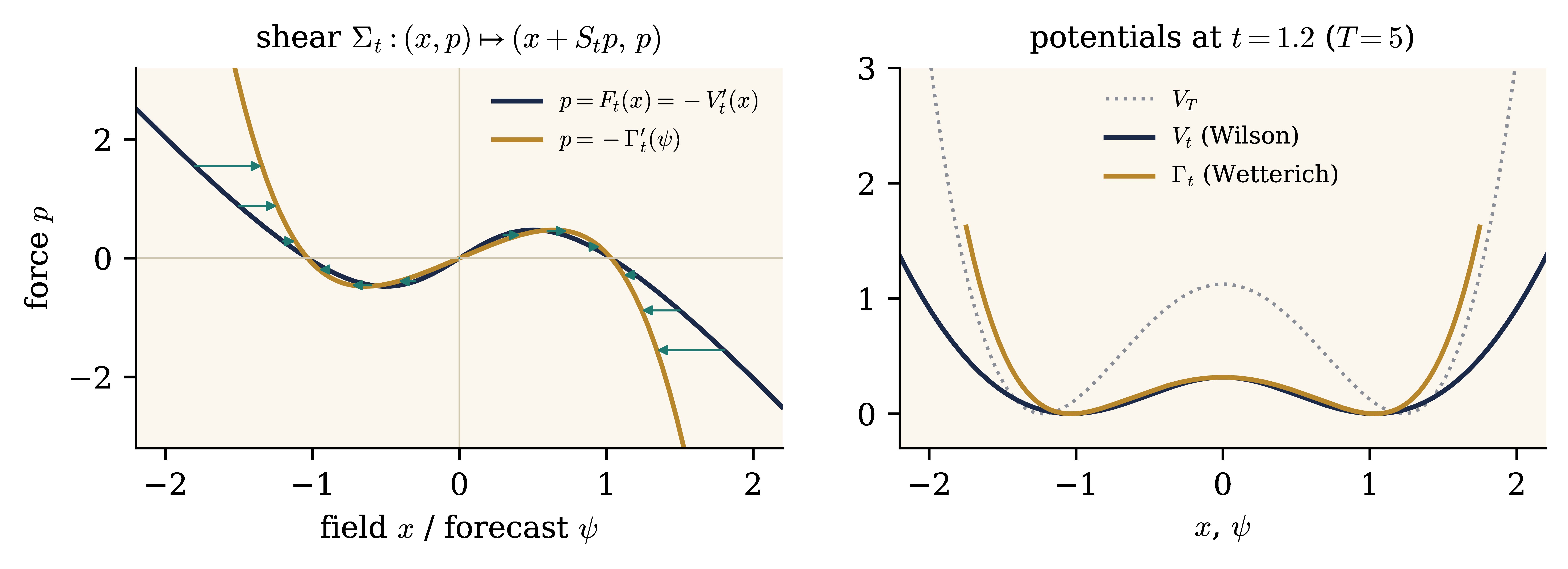
Now let \(F_t = - DV_t\). The graph \(\{(x, - DV_t (x))\}\) is a
Lagrangian submanifold of the (field, force) phase space, and the shear
| \(\displaystyle \mathscr{F}_t = D \Gamma_t, \qquad H_t = (S_t^{- 1} + D^2 \Gamma_t)^{- 1}, \qquad \Gamma_T = V_T .\) | (6.10) |
The generating function of this canonical transformation is the Moreau (infimal convolution) transform
| \(\displaystyle V_t (x) = \inf_{\psi} \left\{ \Gamma_t (\psi) + \tfrac{1}{2} \langle x - \psi, S_t^{- 1} (x - \psi) \rangle \right\},\) | (6.11) |
whose optimality conditions \(x = \psi + S_t D \Gamma_t (\psi)\), \(DV_t
(x) = D \Gamma_t (\psi)\) are
|
Figure 6.2. The zero-dimensional model of Figure 5.2 at \(t = 1.2\). Left: the shear \(\Sigma_t\) (teal arrows) maps the graph of the force \(F_t = - V_t'\) (navy) to a graph over the forecast \(\psi\) (gold), which is the graph of \(- \Gamma_t'\). Right: the bare potential \(V_T\), the effective potential \(V_t\) and \(\Gamma_t\), each shifted to have minimum \(0\). |
Theorem
| \(\displaystyle \partial_t \Gamma_t = \tfrac{1}{2} \text{Tr} [\dot{\mathscr{R}}_t ((S_t^{- 1} + D^2 \Gamma_t)^{- 1} - S_t)], \qquad \Gamma_T = V_T .\) | (6.12) |
Equivalently, the effective average action \(\Gamma^{\text{EAA}}_t (\psi) := \Gamma_t (\psi) + \frac{1}{2} \langle \psi, Q_T^{- 1} \psi \rangle\) solves, up to a field-independent term,
| \(\displaystyle \partial_t \Gamma^{\text{EAA}}_t = \tfrac{1}{2} \text{Tr} [\dot{\mathscr{R}}_t (D^2 \Gamma^{\text{EAA}}_t + \mathscr{R}_t)^{- 1}] .\) | (6.13) |
It interpolates between the bare action \(\Gamma^{\text{EAA}}_T = \frac{1}{2} \langle \psi, Q_T^{- 1} \psi \rangle + V_T (\psi)\) (\(\mathscr{R}_T = \infty\)) and the 1PI effective action \(\Gamma^{\text{EAA}}_0\) of \(\nu_T\) (\(\mathscr{R}_0 = 0\)).
Proof. Integrate
Hence
Thus the Wetterich equation is the gradient-integrated form of the force
equation
Wetterich
FBSDE
field argument \(\psi\)
forecast \(\psi_t =\mathbb{E}_t [\Phi_T]\), the state
transported by \(\Sigma_t\)
\(D \Gamma_t (\psi_t)\)
minus the costate, \(- F_t =\mathbb{E}_t [DV_T
(\Phi_T)]\)
propagator \((D^2 \Gamma^{\text{EAA}}_t +
\mathscr{R}_t)^{- 1}\)
conditional covariance \(\text{Cov}_t\)
regulator \(\mathscr{R}_t = S_t^{- 1} - Q_T^{-
1}\)
precision of the unresolved shell, minus that of the
prior
\(\partial_t \Gamma_t\)
\(\frac{1}{2} \text{Tr} [\dot{\mathscr{R}}_t
(\text{Cov}_t - S_t)]\)
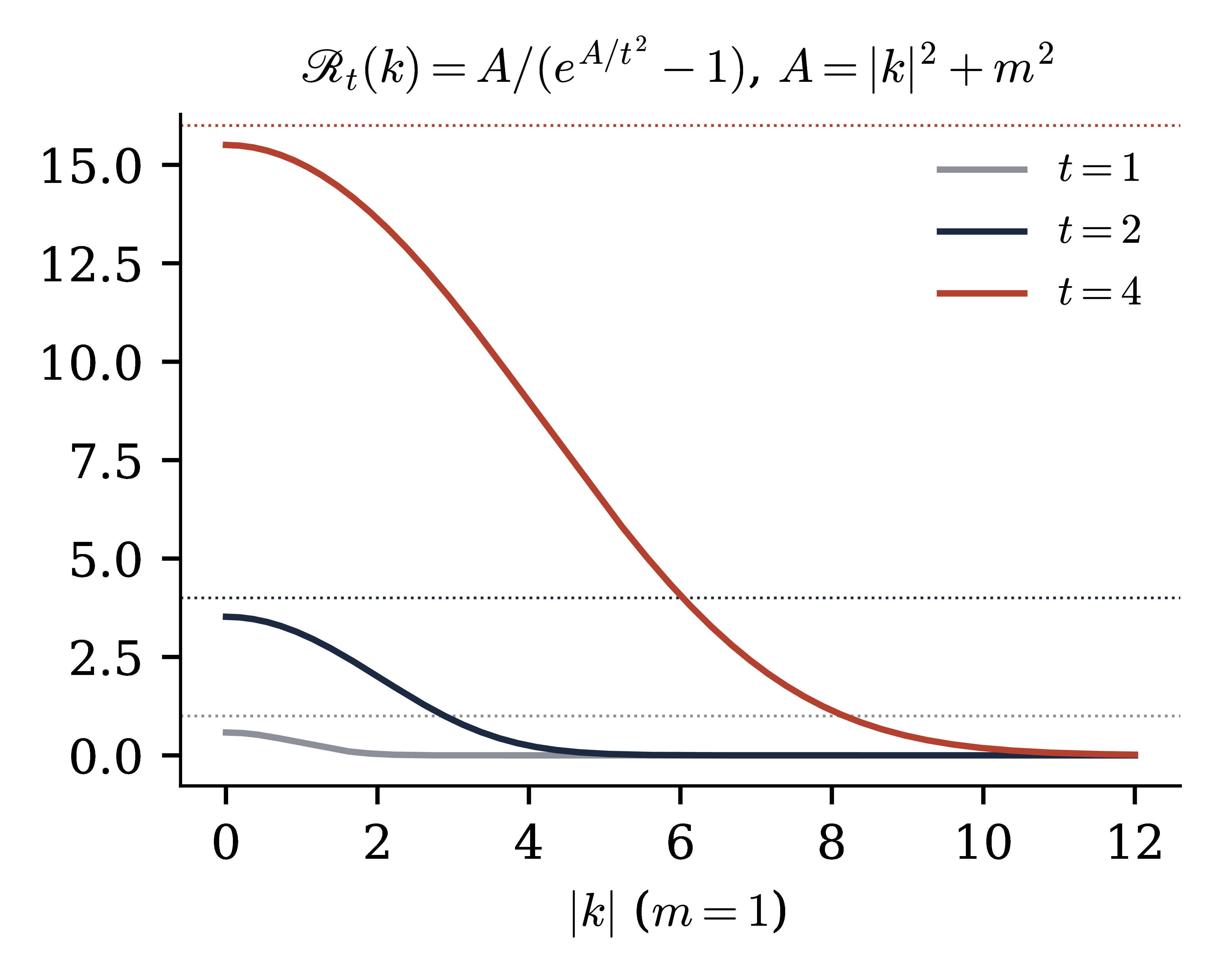
The flow of \(\Gamma\) is driven by the difference between the interacting and the free conditional covariances, paired with the shell \(\dot{\mathscr{R}}_t\). It is one-loop exact, with the full propagator inside the trace. In the Gaussian case \(D^2 \Gamma_t\) is constant and only the constant term of \(\Gamma\) flows. For the heat profile with \(T = \infty\), \(S_t = C (1 - \mathrm{e}^{- A / t^2})\) and
| \(\displaystyle \mathscr{R}_t = \frac{A}{\mathrm{e}^{A / t^2} - 1},\) | (6.14) |
which behaves like a mass term \(t^2\) on the modes \(|k| \ll t\) (for \(m \ll t\)) and is exponentially small on the modes \(|k| \gg t\): the exponential regulator of the functional renormalisation group (Figure 6.3).
| \(\displaystyle \Gamma_t (\psi) = \inf \left\{ \int V_T \hspace{0.17em} \mathrm{d} \nu + \text{Ent} \left( \nu \hspace{0.17em} | \hspace{0.17em} \mu^{S_t} (\cdot - \psi) \right) : \left. \int \varphi \hspace{0.17em} \nu (\mathrm{d} \varphi) = \psi \right\} . \right.\) | (6.15) |
So \(\Gamma_t\), the effective average action up to the quadratic term
\(\frac{1}{2} \langle \psi, Q_T^{- 1} \psi \rangle\), is the free
energy of the unresolved shell constrained to the forecast \(\psi\), and
| \(\displaystyle V^{\text{tree}}_t (x) = \inf_y \left\{ V_T (y) + \tfrac{1}{2} \langle y - x, S_t^{- 1} (y - x) \rangle \right\},\) | (6.16) |
the solution of the noiseless Polchinski equation \(\partial_t V =
\frac{1}{2} \langle DV, \dot{Q} DV \rangle\). It is the saddle point of
the Gaussian convolution
Exercise
Exercise
Exercise
Exercise
Exercise
Exercise
Exercise
Exercise
Exercise
Let \(\mathbb{H}_a\) be the set of progressively measurable drifts \(u : [0, T] \to L^2 (\mathcal{M})\) with \(\mathbb{E} \int_0^T \|u_s \|^2 \mathrm{d} s < \infty\), and set
the field driven by the control \(u\) under the Gaussian reference \(\mathbb{P}_0\).
Theorem
| \(\displaystyle - \log \mathbb{E}_0 [\mathrm{e}^{- V_T (X_T)}] = V_0 (0) = \inf_{u \in \mathbb{H}_a} \mathbb{E}_0 \left[ V_T (X^u_T) + \frac{1}{2} \int_0^T \|u_s \|^2 \mathrm{d} s \right] .\) | (7.1) |
The infimum is attained at the feedback control \(u^{\ast}_s = -
\dot{Q}_s^{1 / 2} DV_s (X^{u^{\ast}}_s)\), and \(\text{Law}
(X^{u^{\ast}}_T) = \nu_T\). The effective potential is the value
function, and
Proof. (Verification.) For any \(u\), by Itô's
formula and
with \(DV_t = DV_t (X^u_t)\) and a martingale \(M\). Integrating and taking expectations,
| \(\displaystyle \mathbb{E}_0 \left[ V_T (X^u_T) + \frac{1}{2} \int_0^T \|u_t \|^2 \mathrm{d} t \right] = V_0 (0) + \frac{1}{2} \mathbb{E}_0 \int_0^T \|u_t + \dot{Q}_t^{1 / 2} DV_t (X^u_t)\|^2 \mathrm{d} t.\) | (7.2) |
So the cost is \(\geq V_0 (0)\), with equality iff \(u = u^{\ast}\).
With this control \(X^{u^{\ast}}\) solves the same SDE as \(\Phi\) in
| \(\displaystyle u_s = - \dot{Q}_s^{1 / 2} \hspace{0.17em} \mathbb{E}_s [DV_T (X^u_T)] = \dot{Q}_s^{1 / 2} F_s .\) | (7.3) |
This is
| \(\displaystyle \mathcal{W}_T (f) := - \log \int \mathrm{e}^{- f} \mathrm{d} \nu_T = \inf_u \mathbb{E}_0 \left[ f (X^u_T) + V_T (X^u_T) + \frac{1}{2} \int_0^T \|u_s \|^2 \mathrm{d} s \right] - V_0 (0) .\) | (7.4) |
Bounds on \(\mathcal{W}_T (f)\) uniform in \(T\), for \(f\) in a rich class, give tightness, moment bounds and the identification of limits. For \(\Phi^4_3\) the naive problem does not have uniform bounds: the leading-order optimal drift \(u_s \approx - 4 \lambda \dot{Q}_s^{1 / 2} : X_s^3\): has a divergent cost. One renormalises by the change of variables \(u = - 4 \lambda \dot{Q}^{1 / 2} : X^3 : + r\). After it, and after further paracontrolled changes of variables, the singular terms are explicit polynomials in the Wick powers of \(X\), cancelled by the counterterms, and the residual functional is coercive. Its control in Besov and paracontrolled norms, uniformly in \(T\), is the construction of \(\Phi^4_3\) in [BG20]; see also [BG21b].
On \(\mathbb{T}^d_L\) the free energy \(V_0 (0)\) and the effective
potential \(V_t\) are extensive: they grow like \(L^d\), and
the force. For a local interaction \(V_T (\varphi) = \int
v_T (\varphi (x)) \mathrm{d} x\), \(DV_T (\varphi) (x) = v_T'
(\varphi (x))\), and
| \(\displaystyle \Phi_t = \int_0^t \dot{Q}_s F_s \hspace{0.17em} \mathrm{d} s + \int_0^t \dot{Q}_s^{1 / 2} \mathrm{d} W_s, \qquad F_t (x) = -\mathbb{E}_t [v_T' (\Phi_T (x))] .\) | (7.5) |
Here every quantity is local, and the equation makes sense without a
volume cutoff. Infinite-volume limits of \(\nu_T^{(L)}\) are
expected to be laws of solutions of
the Burgers flow
differences of free energies. For a local \(f\),
\(\mathcal{W}_T^{(L)} (f)\) in
The coercive estimates must then be local: one uses weighted norms and needs bounds whose constants do not depend on the volume. This infrared problem is the analogue, for the scale dynamics, of the “coming down from infinity” estimates for the parabolic dynamics.
Exercise
Exercise
which diverges linearly in \(T\). Relate this to the \(k
= 4\) term of
The following sections complement the main lecture. They develop the observables of the Gaussian free field and their products, the algebraic and perturbative structure of the Polchinski flow, and the Dyson–Schwinger equations at every scale.
Proposition
is a continuous martingale, with \(\mathrm{d} \hspace{0.17em} : X^n_t : (x) = n \hspace{0.17em} : X^{n - 1}_t : (x) \hspace{0.17em} \mathrm{d} X_t (x)\) and
| \(\displaystyle \mathbb{E} \left[ : X^n_t : (x) \hspace{0.17em} : X^k_t : (y) \right] = \delta_{nk} \hspace{0.17em} n! \hspace{0.17em} Q_t (x, y)^n .\) | (8.1) |
In particular, for \(x \neq y\), \(\lim_t \mathbb{E}[: X^n_t : (x) : X^n_t : (y)] = n! \hspace{0.17em} G (x - y)^n\).
Proof. By Itô's formula, using \(\mathrm{d} \langle X (x), X (x) \rangle_t = \dot{c}_t \hspace{0.17em} \mathrm{d} t\),
The covariance is Lemma 3.8 of Lecture 2, applied to the Gaussian vector \((X_t (x), X_t (y))\).\(\Box\)
Compare with Theorem 3.9 of Lecture 2: there \(: \varphi^n\): existed as a random distribution only for \(n (d - 2) < d\), and by Proposition 3.11 not at all otherwise. As observables, Wick powers exist in every dimension and need no smearing. When \(n (d - 2) \geq d\) and \(0 \leq f \mathrel{\not\equiv} 0\), the smeared martingale \(t \mapsto : X_t^n : (f)\) is unbounded in \(L^2\) and, by the Paley–Zygmund argument of Lecture 2, not even tight as \(t \to \infty\): it has no terminal value, and the observable is the whole family, not a limit. The singularity has not disappeared. It has moved from the observables themselves to their products at coincident points, as we now see.
The pointwise product of two martingales is not a martingale. The natural definition of the product keeps the asymptotics.
Definition
Proposition
| \(\displaystyle \mathbb{E} \int_0^{\infty} | \mathrm{d} \langle O^1, O^2 \rangle_s | < \infty .\) | (8.2) |
Then \(O^1 \star O^2\) exists and
| \(\displaystyle (O^1 \star O^2)_t = O^1_t O^2_t +\mathbb{E}_t \left[ \int_t^{\infty} \mathrm{d} \langle O^1, O^2 \rangle_s \right] .\) | (8.3) |
In particular \(\langle O^1 \star O^2 \rangle = O^1_0 O^2_0 +\mathbb{E} \langle O^1, O^2 \rangle_{\infty}\).
Proof. \(P_t := O^1_t O^2_t - \langle O^1, O^2
\rangle_t\) is a martingale on bounded intervals, and \(N_t :=
\mathbb{E}_t \langle O^1, O^2 \rangle_{\infty}\) is a closed martingale
by
| \(\displaystyle (\textbf{X} (x) \star \textbf{X} (y))_t = X_t (x) X_t (y) + G (x - y) - Q_t (x - y), \qquad \langle \textbf{X} (x) \star \textbf{X} (y) \rangle = G (x - y),\) | (8.4) |
which is the correct two-point function. We never had to discuss the regularity of \(X_{\infty}\). For \(x = y\) and \(d \geq 2\) the product does not exist: its expectation would be \(\lim_t \mathbb{E}X_t (x)^2 = \lim_t c_t = \infty\).
| \(\displaystyle (\textbf{X} (x) \star \textbf{X} (y))_t - G (x - y) \hspace{0.27em} \longrightarrow \hspace{0.27em} X_t (x)^2 - c_t = : X^2_t : (x) .\) | (8.5) |
Since both sides are martingales, this reads \(\textbf{X} (x) \star \textbf{X} (y) = G (x - y) \mathbb{1} + : \textbf{X}^2 : (x) + o (1)\), the remainder tending to zero at each fixed resolution \(t\): the Wick square is the regular part of the product, and \(G (x - y)\) is its singular coefficient. More generally (Exercise 8.2), for \(x \neq y\),
| \(\displaystyle : \textbf{X}^n : (x) \star : \textbf{X}^k : (y) = \sum_{j \leq n \wedge k} j! \binom{n}{j} \binom{k}{j} \hspace{0.17em} G (x - y)^j \hspace{0.17em} : \textbf{X}^{n - j} (x) \textbf{X}^{k - j} (y) :,\) | (8.6) |
where \(: \textbf{X}^p (x) \textbf{X}^q (y) :_t := H_p (X_t (x) ; c_t) H_q (X_t (y) ; c_t)\) minus its contractions at scales \(\leq t\). This is Wick's theorem written at the level of observables. The coefficients \(G (x - y)^j\) carry all the singularities, and the observables on the right have regular limits as \(y \to x\).
Remark
Exercise
Exercise
Exercise
For a positive covariance \(S\) define the renormalisation map
| \(\displaystyle \mathcal{R}_S (V) := - \log (\mu^S \ast \mathrm{e}^{- V}), \qquad (\mu^S \ast u) (\phi) = \int u (\phi + \zeta) \mu^S (\mathrm{d} \zeta) .\) | (9.1) |
Since \(\mu^S \ast \mu^{S'} = \mu^{S + S'}\),
| \(\displaystyle \mathcal{R}_S \circ \mathcal{R}_{S'} =\mathcal{R}_{S + S'} =\mathcal{R}_{S'} \circ \mathcal{R}_S, \qquad V_t =\mathcal{R}_{Q_{T, t}} (V_T) .\) | (9.2) |
So the effective potentials are an orbit of an abelian semigroup, indexed by the cone of positive covariances, acting nonlinearly on interactions and linearly on Boltzmann factors \(\mathrm{e}^{- V}\). Its infinitesimal generators are the vector fields
| \(\displaystyle \mathcal{P}_B (V) := \tfrac{1}{2} \text{Tr} (BD^2 V) - \tfrac{1}{2} \langle DV, BDV \rangle, \qquad \tfrac{\mathrm{d}}{\mathrm{d} s} \mathcal{R}_{sB} (V) |_{s = 0} =\mathcal{P}_B (V),\) | (9.3) |
and
Proposition
Proof. (a) Differentiate \(\mathcal{R}_{sB}
\mathcal{R}_{rB'} =\mathcal{R}_{rB'} \mathcal{R}_{sB}\) at \(s = r =
0\), or compute directly (Exercise 9.1). (b) is
Different profiles with the same endpoints are different coordinate systems on the same renormalisation group trajectory. They change the process \(\Phi\) and the observables at intermediate resolution, but not the terminal theory. The flow has no holonomy [BCG26].
Expanding \(V_t =\mathcal{R}_{Q_{T, t}} (V_T)\) in cumulants of the Gaussian increment \(\zeta \sim \mu^{Q_{T, t}}\) gives
| \(\displaystyle V_t (\phi) =\mathbb{E}_{\zeta} [V_T (\phi + \zeta)] - \tfrac{1}{2} \text{Var}_{\zeta} (V_T (\phi + \zeta)) + \ldots\) | (9.4) |
For
| \(\displaystyle V_t (\phi) = \int [\lambda H_4 (\phi (x) ; c_t) + \gamma_T H_2 (\phi (x) ; c_t)] \mathrm{d} x + O (\lambda^2) .\) | (9.5) |
Here \(\gamma_T = O (\lambda^2)\) is kept for later use. At first order the effective potential is the Wick-ordered potential at the current resolution. This is the dual statement of Proposition 8.1: \(\int H_4 (X_t ; c_t)\) is an observable.
Proposition
| \(\displaystyle V_t (\phi) = \int [\lambda : \phi^4 :_t + \gamma_T : \phi^2 :_t] - \frac{\lambda^2}{2} \sum_{k = 1}^4 \binom{4}{k}^2 k! \iint S (x, y)^k \hspace{0.17em} : \phi^{4 - k} :_t (x) \hspace{0.17em} : \phi^{4 - k} :_t (y) \hspace{0.17em} \mathrm{d} x \hspace{0.17em} \mathrm{d} y + O (\lambda^3) .\) | (9.6) |
Proof. By the binomial formula for Hermite polynomials,
Then compute the variance in
Now let \(T \to \infty\) at fixed \(t\), so that \(S \to C - Q_t\), which near the diagonal is as singular as \(G\). In \(d = 2\) every \(S^k\) is locally integrable, so with \(\gamma_T = 0\) every term has a limit: Wick ordering suffices. In \(d = 3\), \(G (z) \sim (4 \pi |z|)^{- 1}\):
\(k = 1, 2\): \(S\) and \(S^2\) are locally integrable. These terms are finite and nonlocal.
\(k = 3\) (the sunset): \(S^3 \sim |z|^{- 3}\) is not integrable. Writing \(\phi (x) \phi (y) = \frac{1}{2} (\phi (x)^2 + \phi (y)^2) - \frac{1}{2} (\phi (x) - \phi (y))^2\), up to a field-independent constant the divergent part is local: \(- 48 \lambda^2 \left( \int S^3 \right) \int : \phi^2 :_t +\)(finite), with \(\int S^3 \sim \frac{1}{16 \pi^2} \log T\). It is cancelled by
| \(\displaystyle \gamma_T := 48 \lambda^2 \int_{\mathbb{T}^3_L} Q_T (z)^3 \hspace{0.17em} \mathrm{d} z = \frac{3 \lambda^2}{\pi^2} \log T + O (1),\) | (9.7) |
since \(\gamma_T - 48 \lambda^2 \int S^3\) converges (Exercise 9.2).
\(k = 4\): a divergent constant \(- 12 \lambda^2 L^3 \int S^4 \sim T\), the vacuum energy. It cancels in \(\nu_T\) but not in the free energy.
Power counting (Exercise 9.3) shows that no further field-dependent counterterms are needed in \(d = 3\): \(\Phi^4_3\) is superrenormalisable. Thus renormalisation appears as a property of the flow: one chooses the terminal data \(V_T\) so that the effective potentials \(V_t\) at fixed resolution have limits. The divergences at second order are also related to the singularity of \(\Phi^4_3\) with respect to the GFF [BG21b]: the measures \(\nu_t\) at fixed \(t\) are expected to stay absolutely continuous with respect to \(\mu^{Q_t}\), while the terminal one is not.
Exercise
Exercise
Exercise
Assume now that all the operators involved are functions of \(A\), hence commute, and let
For the heat profile, \(K = A \mathrm{e}^{A / T^2}\) and \(J_t = \mathrm{e}^{- A (t^{- 2} - T^{- 2})}\) is a heat semigroup, which tends to \(\mathrm{e}^{- A / t^2}\) as \(T \to \infty\). \(F_t\) is the force observable of Theorem 5.4.
Theorem
| \(\displaystyle \eta_t := K \Phi_t - J_t F_t\) | (10.1) |
is a centred \(\mathbb{P}\)-martingale, with \(\mathrm{d} \eta_t = K \dot{Q}_t^{1 / 2} \mathrm{d} W^{\mathbb{P}}_t - J_t \hspace{0.17em} \mathrm{d} F_t\). For every \(t \leq T\), every \(h\) and every functional \(G\),
| \(\displaystyle \mathbb{E}^{\mathbb{P}} [D_{J_t h} G (\Phi_t)] =\mathbb{E}^{\mathbb{P}} \left[ G (\Phi_t) \hspace{0.17em} \langle h, \eta_t \rangle \right] =\mathbb{E}^{\mathbb{P}} \left[ G (\Phi_t) \hspace{0.17em} \langle h, K \Phi_t - J_t F_t \rangle \right] .\) | (10.2) |
At \(t = T\) this is the Dyson–Schwinger equation of \(\nu_T\),
| \(\displaystyle \mathbb{E}^{\nu_T} [D_h G] =\mathbb{E}^{\nu_T} \left[ G \hspace{0.17em} \langle h, K \varphi + DV_T (\varphi) \rangle \right] .\) | (10.3) |
Proof. From
Formally letting \(T \to \infty\), \(K \to A\), and
| \(\displaystyle A \Phi_t = AQ_t \hspace{0.17em} F_t + \eta_t,\) | (10.4) |
with \(AQ_t = \mathrm{e}^{- A / t^2}\) for the heat profile. This is the
Euclidean field equation \(A \varphi = - V' (\varphi) +\)noise of
Lectures 1–2, seen at resolution \(t\). It needs no products of
distributions: the nonlinearity enters only through the force
observable \(F_t\), smeared at scale \(1 / t\). For the GFF
(\(F = 0\)),
Remark
Exercise
Exercise
S. Albeverio, S. Liang, B. Zegarlinski. Remark on the integration by parts formula for the \(\varphi^4_3\)-quantum field model. Infin. Dimens. Anal. Quantum Probab. Relat. Top. 9 (2006), 149–154.
R. Bauerschmidt, T. Bodineau, B. Dagallier. Stochastic dynamics and the Polchinski equation: an introduction. Probab. Surveys 21 (2024), 200–290.
R. Bauerschmidt, D.C. Brydges, G. Slade. Introduction to a Renormalisation Group Method. Lecture Notes in Math. 2242, Springer, 2019.
J. Berges, N. Tetradis, C. Wetterich. Non-perturbative renormalization flow in quantum field theory and statistical physics. Phys. Rep. 363 (2002), 223–386.
I. Bailleul, I. Chevyrev, M. Gubinelli. Stochastic observables and Wilson–Itô diffusions. In preparation.
M. Boué, P. Dupuis. A variational representation for certain functionals of Brownian motion. Ann. Probab. 26 (1998), 1641–1659.
N. Barashkov, M. Gubinelli. A variational method for \(\Phi^4_3\). Duke Math. J. 169 (2020), 3339–3415.
N. Barashkov, M. Gubinelli. The \(\Phi^4_3\) measure via Girsanov's theorem. Electron. J. Probab. 26 (2021), 1–29.
N. Barashkov, M. Gubinelli. On the variational method for Euclidean quantum fields in infinite volume. Probab. Math. Phys. 4 (2023), 761–801.
D.C. Brydges, T. Kennedy. Mayer expansions and the Hamilton–Jacobi equation. J. Stat. Phys. 48 (1987), 19–49.
R. Eldan. Analysis of high-dimensional distributions using pathwise methods. In Proceedings of the ICM 2022, EMS Press, 2023, 4246–4270.
M. Gubinelli, M. Hofmanová. A PDE construction of the Euclidean \(\Phi^4_3\) quantum field theory. Comm. Math. Phys. 384 (2021), 1–75.
J. Glimm, A. Jaffe, T. Spencer. Phase transitions for \(\varphi^4_2\) quantum fields. Comm. Math. Phys. 45 (1975), 203–216.
T.R. Morris. The exact renormalization group and approximate solutions. Int. J. Mod. Phys. A 9 (1994), 2411–2449.
J. Ma, J. Yong. Forward-Backward Stochastic Differential Equations and their Applications. Lecture Notes in Math. 1702, Springer, 1999.
J. Polchinski. Renormalization and effective Lagrangians. Nuclear Phys. B 231 (1984), 269–295.
M. Salmhofer. Renormalization: An Introduction. Springer, 1999.
C. Wetterich. Exact evolution equation for the effective potential. Phys. Lett. B 301 (1993), 90–94.
K.G. Wilson, J. Kogut. The renormalization group and the \(\epsilon\) expansion. Phys. Rep. 12 (1974), 75–199.