Constructive quantum field theory — Lecture 1 (notes)

Introduction

Constructive quantum field theory aims at constructing, with full mathematical rigour, examples of interacting relativistic quantum fields, i.e. models satisfying a small set of axioms which encode quantum mechanics, special relativity and causality. In spacetime dimension \(d = 2\) and \(d = 3\) this programme has been carried out for several models (\(P (\varphi)_2\), Yukawa_\(2\), \(\Phi^4_3\), sine-Gordon, …), while in \(d = 4\) no interacting model is known, and the scaling limits of critical lattice \(\varphi^4_4\) models are Gaussian (trivial) [ADC21].

The main lesson of the late 1960s and 1970s [Sym69, Nel73a, Nel73b, OS73, OS75, GRS75] is that it is much more efficient to work in imaginary time. The relativistic theory is then encoded in a probability measure on distributions on \(\mathbb{R}^d\), which looks like the continuum limit of a classical lattice spin system at a critical point. All modern approaches (cluster expansions, renormalisation group, stochastic quantisation, variational methods) work at this Euclidean level.

Plan.

Conventions.

1Relativistic quantum fields in Minkowski space

1.1Kinematics

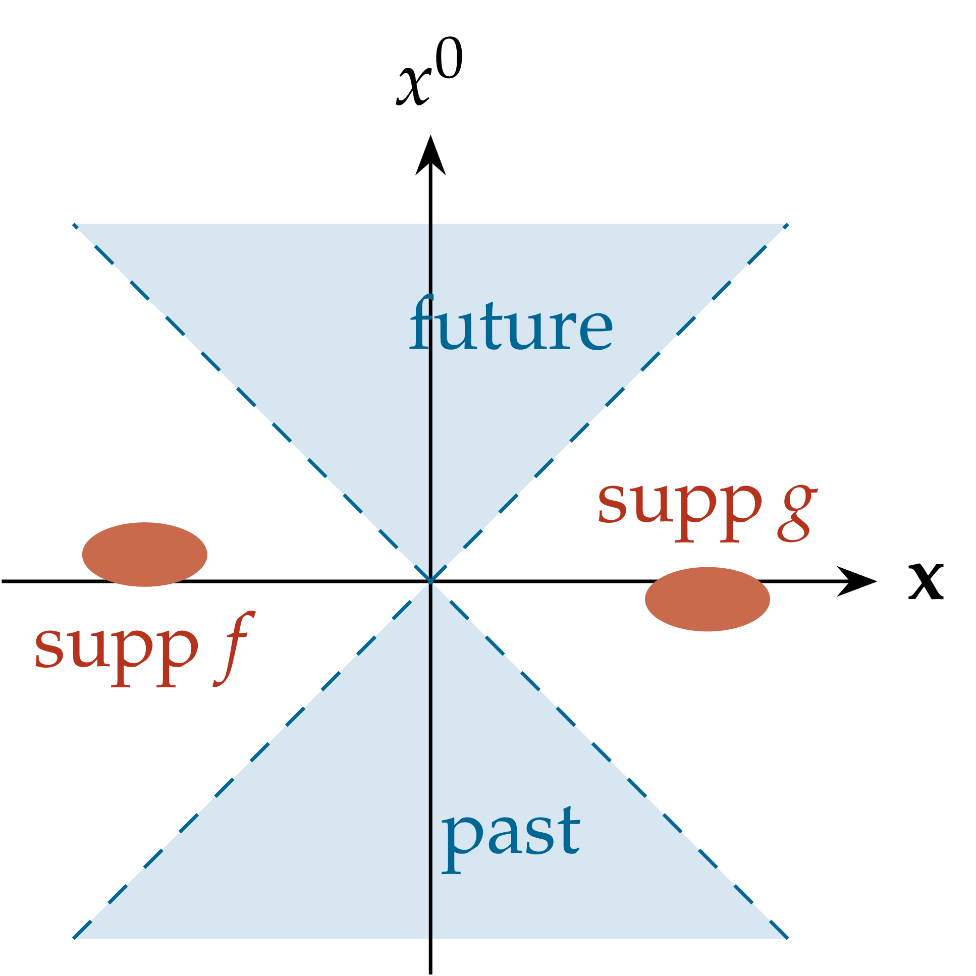
Minkowski space is \(\mathbb{R}^{1, s} \simeq \mathbb{R}^d\) with points \(x = (x^0, \textbf{x})\) and bilinear form \(x \cdot y = x^0 y^0 - \textbf{x} \cdot \textbf{y}\), \(x^2 = x \cdot x\). Two points are spacelike separated if \((x - y)^2 < 0\). The open forward light cone is \(V_{\hspace{-0.17em} +} = \{p : \hspace{0.17em} p^0 > | \textbf{p} |\}\), with closure \(\bar{V}_{\hspace{-0.17em} +}\). The restricted Lorentz group \(\mathcal{L}^{\uparrow}_+\) is the connected component of the identity of the group of linear maps preserving \(x \cdot y\); the restricted Poincaré group is \(\mathcal{P}^{\uparrow}_+ =\mathbb{R}^d \rtimes \mathcal{L}^{\uparrow}_+\), with \((a, \Lambda) (b, \Lambda') = (a + \Lambda b, \Lambda \Lambda')\), acting on spacetime by \(x \mapsto \Lambda x + a\).

Figure 1.1. Minkowski space for \(s = 1\). The shaded regions are timelike to the origin. The supports of \(f\) and \(g\) are spacelike separated, so \([\varphi (f), \varphi (g)] = 0\) by (W3). In momentum space the same forward cone \(\bar{V}_{\hspace{-0.17em} +}\) carries the joint spectrum of \((H, \textbf{P})\).

By Wigner's theorem a relativistic quantum system carries a (projective) unitary representation of \(\mathcal{P}^{\uparrow}_+\) on its Hilbert space of states. For a scalar field we may assume a true representation.

1.2The Wightman axioms

Definition 1.1. (Wightman QFT of a hermitian scalar field) A Wightman theory is given by the following data, subject to the following conditions.

Formally \(\varphi (f) = \int \varphi (x) f (x) \hspace{0.17em} \mathrm{d} x\), and \(\varphi (x^0, \textbf{x}) = \mathrm{e}^{\mathrm{i} Hx^0} \varphi (0, \textbf{x}) \mathrm{e}^{- \mathrm{i} Hx^0}\) is the Heisenberg-picture field. For \(d \geq 3\), Lorentz invariance of the vacuum follows from translation invariance and uniqueness: \(U (0, \Lambda) \Omega\) is translation invariant, hence equal to \(\chi (\Lambda) \Omega\) for a character \(\chi\) of \(\mathcal{L}^{\uparrow}_+\), and \(\chi \equiv 1\) because \(\mathcal{L}^{\uparrow}_+\) has no nontrivial one-dimensional unitary representations. For \(d = 2\) the boosts form the abelian group \(\mathbb{R}\); there one may always replace \(U (a, \Lambda)\) by \(\chi (\Lambda)^{- 1} U (a, \Lambda)\), which is why we include Lorentz invariance in (W0). The Wightman functions

extend, by the Schwartz kernel theorem, to tempered distributions \(W_n \in \mathcal{S}' (\mathbb{R}^{dn})\). They satisfy: (a) positivity: \(\sum_{j, k} W_{j + k} (g_j^{\ast} \otimes g_k) \geq 0\) for every finite sequence \(g_j \in \mathcal{S} (\mathbb{R}^{dj})\), with \(g^{\ast} (x_1, \ldots, x_j) = \overline{g (x_j, \ldots, x_1)}\); (b) Poincaré invariance; (c) spectral condition: \(W_n (x_1, \ldots, x_n) = w_n (x_1 - x_2, \ldots, x_{n - 1} - x_n)\) with \(\hat{w}_n\) supported in \(\bar{V}_{\hspace{-0.17em} +}^{\hspace{0.17em} n - 1}\) (for a suitable sign convention); (d) locality: \(W_n\) is unchanged under exchange of two adjacent spacelike separated arguments; (e) cluster property, equivalent to uniqueness of the vacuum (Remark 2.7).

Theorem 1.2. (Wightman reconstruction [SW64]) Any sequence \((W_n)_{n \geq 0}\) of tempered distributions with \(W_0 = 1\) satisfying (a)–(d) is the sequence of Wightman functions of a theory satisfying (W1)–(W4) and (W0) except possibly uniqueness of the vacuum, unique up to unitary equivalence. The vacuum is unique iff (e) holds.

So constructing a QFT amounts to constructing its Wightman functions. For the axioms, the reconstruction theorem and the algebraic viewpoint see [SW64, BSZ92, Haa96]. The difficulty is that the positivity condition (a) is hard to verify for candidate Wightman functions: it involves all \(W_n\) at once, and the objects one can actually construct live in imaginary time, whereas (a) refers to their real-time boundary values. The Euclidean approach of Section 2 replaces it by reflection positivity, which can be checked on regularised (e.g. lattice) approximations and is preserved under the limits one has to take. Note also that the axioms say nothing about dynamics: there is no Lagrangian, and the interaction is hidden in the higher Wightman functions.

Remark 1.3. (Minimal requirements) The axioms (W0)–(W4) are a minimal transcription of what we expect of any relativistic quantum theory with a local quantity. (W0) encodes quantum mechanics (states in a Hilbert space), Poincaré symmetry (Wigner's theorem), and stability: the energy is bounded below, which together with Lorentz covariance gives the spectrum condition, and there is a ground state. (W1) and (W2) require a covariant quantity localised in spacetime regions. (W3) is Einstein causality: measurements in spacelike separated regions do not interfere. (W4) says that the field is complete: all states are produced from the vacuum by local operations. Nothing is assumed about dynamics, Lagrangians, perturbation theory or particles. These either follow as theorems (PCT and the spin–statistics connection [SW64]; particles and scattering states from an isolated mass shell, by Haag–Ruelle theory [Haa96]) or are additional structure. A construction of a relativistic QFT must at least produce a model of these axioms, which is why they are our target. They are often supplemented by the time-slice axiom (primitive causality): the fields smeared in an arbitrarily thin time slice already generate all operators. It expresses the existence of a dynamical law and is the abstract counterpart of a well-posed Cauchy problem [Haa96, §II.1].

Remark 1.4. (Local algebras and fields) For a bounded open region \(O \subset \mathbb{R}^d\), let \(\mathfrak{A} (O)\) be the von Neumann algebra generated by the bounded functions of the smeared fields \(\varphi (f)\), \(f\) real with \(\text{supp} f \subset O\). (This requires the closures of the \(\varphi (f)\) to be self-adjoint and to commute strongly at spacelike separation, which holds in the models we construct.) The map \(O \mapsto \mathfrak{A} (O)\) is a Haag–Kastler net [HK64, Haa96]. It satisfies isotony, \(\mathfrak{A} (O_1) \subset \mathfrak{A} (O_2)\) for \(O_1 \subset O_2\); Einstein causality, \([\mathfrak{A}(O_1), \mathfrak{A}(O_2)] = 0\) for spacelike separated regions; covariance, \(U (a, \Lambda) \mathfrak{A} (O) U (a, \Lambda)^{\ast} =\mathfrak{A} (\Lambda O + a)\); and the spectrum condition, with a vacuum vector. In the algebraic point of view the net is the physical content of the theory: it specifies which observables can be measured in each region, and nothing else. A field is a choice of coordinates for the net. Different fields can generate the same net, and fields that are local relative to each other (the Borchers class of \(\varphi\), which contains for instance all Wick polynomials of a free field) describe the same physics, e.g. the same scattering matrix. Conversely, fields need not be observable: fermion fields anticommute at spacelike separation, and charged fields are not invariant under the gauge group.

We nevertheless need fields, for three reasons. (a) The net refers to regions, not to points. Fields provide the pointlike localised quantities in which dynamics (field equations, Lagrangians), interactions (local products such as \(: \varphi^4\):) and the short-distance structure (operator product expansion, scaling dimensions) are expressed. (b) Correlation functions of fields are the concrete objects that constructive methods produce and estimate: the Euclidean measures of these lectures. (c) The two descriptions are close but not equivalent. The Wightman axioms alone do not guarantee a net of local algebras of bounded operators, and a net does not guarantee a Wightman field [Haa96, §III.1]. Under a phase-space condition, Fredenhagen and Hertel recover pointlike localised fields from a net by shrinking the regions to points [FH81]. In this course a QFT is constructed as a Euclidean measure for a field, and its local algebras are those generated by the reconstructed field.

Remark 1.5. (The vacuum, and states without a vacuum) In Minkowski space the vacuum is singled out by symmetry and stability: it is the Poincaré invariant state, and by the spectrum condition it has the lowest energy in every Lorentz frame. In the Wightman framework its existence is an axiom. In the constructive approach it is a result: it arises as the limit \(T \to \infty\) of the Euclidean measures (Table 2.1), and its uniqueness is equivalent to clustering (Remark 2.7). On a curved spacetime, for instance an expanding Friedmann–Robertson–Walker universe, there is no Poincaré group. Without a timelike Killing field there is neither a conserved energy nor a preferred vacuum, and the notion of particle becomes observer dependent (particle creation in expanding universes, and in gravitational collapse, the Hawking effect; already in flat space, the Unruh effect shows that the notion of particle depends on the observer). The algebraic framework still makes sense: nets of local algebras can be defined locally and covariantly [BFV03]. But the physically acceptable states must be selected by a local condition, the Hadamard condition: at short distance, the two-point function has the same singularity as the Minkowski vacuum. In \(d = 4\) it reads, schematically,

where \(\sigma (x, y)\) is the squared geodesic distance, taken positive at spacelike separation (so that \(W_2 = 1 / (4 \pi^2 \sigma_{\varepsilon})\) for the massless field in Minkowski space), and \(\sigma_{\varepsilon} (x, y) = \sigma (x, y) + 2 \mathrm{i} \varepsilon (t (x) - t (y)) + \varepsilon^2\), \(\varepsilon \downarrow 0\), implements the positive-frequency \(\mathrm{i} \varepsilon\) prescription (\(t\) a time function), the coefficients \(U, V\) are determined by the metric and the field equation, and \(w\) is smooth and state dependent. By Radzikowski's theorem this is equivalent to a microlocal spectrum condition: the wave front set of \(W_2\) contains only positive frequencies [Rad96]. This is the local substitute for positivity of the energy. Hadamard states are the states in which Wick powers and the expectation of the stress–energy tensor can be renormalised, by subtracting the geometric part of \(W_2\) (point splitting). This is what semiclassical gravity and cosmology need [Wal94]; examples are the Bunch–Davies state of de Sitter space, used for inflationary perturbations, and the states of low energy on Friedmann–Robertson–Walker spacetimes (adiabatic states of finite order are, in general, only approximately Hadamard). In the language of these lectures, Remark 1.10(iii) and its Euclidean version (Remark 3.7) show that in flat space every theory is at least as singular as the free field. The Hadamard condition prescribes exactly the free singularity, and the Wick ordering of Lecture 2 is the flat-space version of the subtraction of the Hadamard parametrix.

1.3Why operator-valued distributions?

The free field.

For \(f \in \mathcal{S} (\mathbb{R}^d)\) one gets \(\varphi (f) \Omega = a^{\ast} (\tilde{f}) \Omega\) with \(\tilde{f} (\textbf{p}) = \int f (x) \mathrm{e}^{\mathrm{i} p \cdot x} \mathrm{d} x|_{p^0 = \omega (\textbf{p})}\), and

But formally \(\| \varphi (x) \Omega \|^2 = W_2 (0) = \int \mathrm{d} \Omega_m = + \infty\) for \(s \geq 1\): field fluctuations at a point are infinite. The divergence is ultraviolet (large momenta). It is logarithmic for \(s = 1\) and power-like for \(s \geq 2\). This is not an artefact of the free field.

Proposition 1.6. (No fields at a point; Wightman [Wig64]) Assume (W0)–(W2) and suppose there is \(\psi \in \mathcal{H}\) such that \(\varphi (f) \Omega = \int f (x) U (x, \mathbb{1}) \psi \hspace{0.17em} \mathrm{d} x\) for all \(f \in \mathcal{S} (\mathbb{R}^d)\), i.e. “\(\varphi (0) \Omega = \psi\) exists”. Then \(\psi = \langle \Omega, \psi \rangle \Omega\), hence \(\varphi (f) \Omega = \langle \Omega, \psi \rangle \left( \int f \right) \Omega\).

Lemma 1.7. Let \(d \geq 2\) and let \(\mu\) be a finite positive Borel measure on \(\bar{V}_{\hspace{-0.17em} +}\) invariant under \(\mathcal{L}^{\uparrow}_+\). Then \(\mu = \mu (\{0\}) \delta_0\).

Proof. A boost of rapidity \(\theta\) in the \(x^1\) direction acts as \(p^0 \pm p^1 \mapsto \mathrm{e}^{\pm \theta} (p^0 \pm p^1)\), leaving the other components unchanged. Let \(S^{\pm}_j = \{p \in \bar{V}_{\hspace{-0.17em} +} : \hspace{0.17em} 2^j \leq p^0 \pm p^1 < 2^{j + 1} \}\), \(j \in \mathbb{Z}\). The boost with \(\mathrm{e}^{\theta} = 2\) maps \(S^+_j\) onto \(S^+_{j + 1}\), so \(\mu (S^+_j)\) is independent of \(j\). These sets are disjoint and \(\mu\) is finite, so \(\mu (S^+_j) = 0\). The same argument applies to \(S^-_j\). Finally \(\bigcup_j (S^+_j \cup S^-_j) = \bar{V}_{\hspace{-0.17em} +} \setminus \{0\}\), since \(p^0 \pm p^1 \geq 0\) on \(\bar{V}_{\hspace{-0.17em} +}\) and \(p^0 + p^1 = p^0 - p^1 = 0\) forces \(p = 0\).\(\Box\)

Proof of Proposition 1.6. By covariance, \(U (0, \Lambda) \varphi (f) \Omega = \varphi (f_{(0, \Lambda)}) \Omega\). Since \(U (0, \Lambda) U (x, \mathbb{1}) = U (\Lambda x, \mathbb{1}) U (0, \Lambda)\), after the change of variables \(x \mapsto \Lambda x\) this reads

Letting \(f \to \delta_0\) gives \(U (0, \Lambda) \psi = \psi\). Let \(\mu\) be the spectral measure of \(\psi\) for the translations, \(\langle \psi, U (a, \mathbb{1}) \psi \rangle = \int \mathrm{e}^{\mathrm{i} p \cdot a} \mu (\mathrm{d} p)\). It is finite with mass \(\| \psi \|^2\), supported in \(\bar{V}_{\hspace{-0.17em} +}\) by the spectrum condition, and Lorentz invariant because \(\psi\) is. By Lemma 1.7, \(\langle \psi, U (a, \mathbb{1}) \psi \rangle = \| \psi \|^2\) for all \(a\), hence \(U (a, \mathbb{1}) \psi = \psi\) (equality in Cauchy–Schwarz), and \(\psi \in \mathbb{C} \Omega\) by uniqueness of the vacuum.\(\Box\)

Remark 1.8. So the only theories with point-like fields have \(\varphi (f) \Omega \propto \Omega\); using locality and the Reeh–Schlieder theorem one then shows that \(\varphi\) is a multiple of the identity [SW64, Wig64]. Physically (Bohr–Rosenfeld), measuring a field at a sharp point requires infinite energy. Quantum fields are therefore operator-valued distributions, and every nonlinear expression in \(\varphi (x)\) (interaction terms, field equations, composite operators) requires a definition. This is the root of renormalisation.

1.4The two-point function: the Källén–Lehmann representation

The free two-point function (1.3) is the Fourier transform of the invariant measure on the mass shell. In every Wightman theory the two-point function is a positive superposition of such free ones. For \(M \geq 0\) let \(W_2^{(M)}\) be the two-point function (1.3) of the free field of mass \(M\). For \(M = 0\) and \(d \geq 3\) it is defined with the invariant measure \(\mathrm{d} \Omega_0 = \mathrm{d} \textbf{p} / ((2 \pi)^s 2| \textbf{p} |)\) on the boundary of the cone; for \(d = 2\) the measure \(\mathrm{d} p / |p|\) is not locally finite at \(p = 0\), and \(W_2^{(0)}\) is not defined. By translation invariance of \(\Omega\), \(\langle \Omega, \varphi (f) \Omega \rangle = v \int f\) for some \(v \in \mathbb{R}\).

Theorem 1.9. (Källén–Lehmann [Kal52, Leh54]) Assume (W0)–(W2). There is a positive Borel measure \(\rho\) on \([0, \infty)\), the spectral measure of the field, such that

in the sense of tempered distributions. The measure \(\rho\) grows at most polynomially and is such that the right-hand side is tempered; in particular \(\rho (\{0\}) = 0\) if \(d = 2\).

Sketch. Let \(\psi_f := \varphi (f) \Omega - v (\int f) \Omega \perp \Omega\). By hermiticity \(\langle \psi_{\bar{f}}, \psi_g \rangle = W_2 (f \otimes g) - v^2 \int f \int g\), and by covariance \(U (a, \mathbb{1}) \psi_f = \psi_{f_{(a, \mathbb{1})}}\). Hence the truncated function \(W_2^T := W_2 - v^2\) is a distribution of positive type in \(x - y\). By the Bochner–Schwartz theorem (equivalently, the spectral theorem for the translations restricted to the closed span of the \(\psi_f\)) it is the Fourier transform of a positive tempered measure \(\mu\) on momentum space. The spectrum condition gives \(\text{supp} \mu \subset \bar{V}_{\hspace{-0.17em} +}\). Since \(\psi_f \perp \Omega\) and \(\Omega\) is the only translation invariant vector, \(\mu (\{0\}) = 0\). Covariance and \(U (0, \Lambda) \Omega = \Omega\) make \(\mu\) invariant under \(\mathcal{L}^{\uparrow}_+\). The \(\mathcal{L}^{\uparrow}_+\)-orbits in \(\bar{V}_{\hspace{-0.17em} +} \setminus \{0\}\) are the hyperboloids \(H^+_M\), \(M > 0\), and (for \(d \geq 3\)) the punctured boundary of the cone, \(M = 0\). Each carries a unique invariant measure up to normalisation, namely \(\mathrm{d} \Omega_M\). (For \(d = 2\) the two half-lines \(p^0 = \pm p^1 > 0\) of the cone boundary are orbits too, but their invariant measures \(\mathrm{d} p^{\pm} / p^{\pm}\) are not locally finite at \(0\), so a tempered \(\mu\) cannot charge them; hence \(\rho (\{0\}) = 0\).) Disintegrating \(\mu\) along \(M = (p^2)^{1 / 2}\) gives \(\mu = \int \rho (\mathrm{d} M^2) \hspace{0.17em} \Omega_M\), which is (1.4).\(\Box\)

Remark 1.10. (Reading the spectrum off \(\rho\)) (i) Free fields. The free field has \(\rho = \delta_{m^2}\). Conversely, if \(\rho = \delta_{m^2}\) with \(m > 0\) then \(\varphi - v\) is a free field of mass \(m\) (Jost–Schroer theorem [SW64]; it uses the full Wightman axioms, in particular locality (W3)). So an interacting theory must have \(\rho \neq \delta_{m^2}\); this is not sufficient, since generalised free fields have arbitrary \(\rho\) and no interaction (Exercise 1.6).

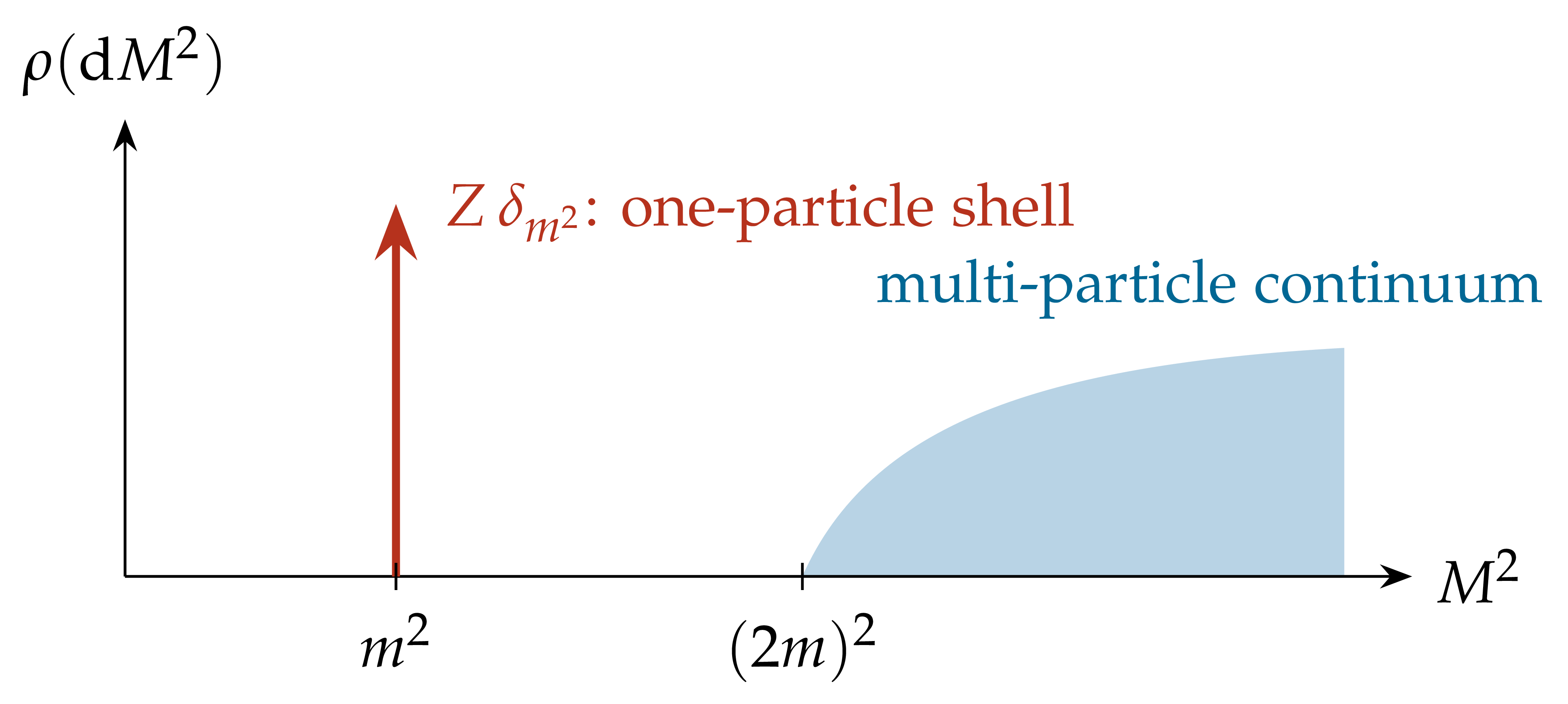
(ii) Particles. An atom \(Z \delta_{m^2}\) of \(\rho\) isolated from the rest of its support, \(Z > 0\), signals a particle of mass \(m\): an isolated eigenvalue \(m\) of the mass operator \((H^2 - \textbf{P}^2)^{1 / 2}\). The remaining part of \(\rho\) describes multi-particle states. In the absence of bound states it starts at \((2 m)^2\), or at \((3 m)^2\) if the theory is invariant under \(\varphi \mapsto - \varphi\). For weakly coupled \(P (\varphi)_2\) models the isolated one-particle shell was established in [GJS74].

(iii) No point fields, again. Formally \(W_2^T (0) = \int \rho (\mathrm{d} M^2) \int \mathrm{d} \Omega_M = \infty\) for any \(\rho \neq 0\) when \(d \geq 2\). The singularity at coincident points of a nontrivial Wightman field is at least as strong as that of the free field. Remark 3.7 gives a precise Euclidean version of this statement.

(iv) Canonical fields and field-strength renormalisation. If the sharp-time fields exist and satisfy the CCR (1.6), then \(\int \rho (\mathrm{d} M^2) = 1\) (Exercise 1.5). Hence \(Z = \rho (\{m^2 \}) \leq 1\), with equality iff \(\rho = \delta_{m^2}\). The time-zero fields of \(P (\varphi)_2\) models satisfy the CCR [GJ87]. In \(d = 4\), perturbation theory gives \(\int \rho = \infty\), i.e. “\(Z = 0\)”: the renormalised field cannot be canonical, and must be rescaled by a divergent factor (wave-function renormalisation).

Figure 1.2. Typical spectral measure of an interacting field with mass gap (Theorem 1.9 and Remark 1.10): an isolated atom at the one-particle mass (\(0 < Z \leq 1\) for a canonical field), and a continuum starting at \((2 m)^2\), or at \((3 m)^2\) in the presence of the symmetry \(\varphi \mapsto - \varphi\). The free field has \(\rho = \delta_{m^2}\).

1.5The quantum wave equation

Since \((- p^2 + m^2) \mathrm{e}^{\pm \mathrm{i} p \cdot x} = 0\) on the mass shell, the free field (1.2) solves the Klein–Gordon equation in the sense of distributions:

Moreover, the sharp-time fields \(\varphi (t, g) = \int \varphi (t, \textbf{x}) g (\textbf{x}) \mathrm{d} \textbf{x}\) and \(\pi (t, g)\), with \(\pi = \partial_t \varphi\), are well defined for \(g \in \mathcal{S} (\mathbb{R}^s)\) (Exercise 1.3), and satisfy the canonical commutation relations (CCR)

One may think of \(\varphi\) as the solution of a linear wave equation with quantum initial data: \((\varphi (0, \cdot), \pi (0, \cdot))\) satisfy the CCR and are “distributed” according to the vacuum.

Free field on a spatial circle.

The free field is an infinite collection of independent harmonic oscillators, one per mode. With an ultraviolet cutoff \(|k| \leq R\),

Interactions.

together with the CCR (1.6). This immediately runs into three problems.

1. \(\varphi (x)^3\) has no meaning, being the cube of a distribution. It must be renormalised. In \(d = 2\) Wick ordering \(: \varphi^3\): suffices (cf. (1.8) and Section 3.3); in \(d = 3\) a further mass counterterm is needed in the equation (and a vacuum-energy counterterm in the Hamiltonian); in \(d = 4\) the theory is expected to be trivial, as is proved for the scaling limits of critical lattice \(\varphi^4_4\) models [ADC21].

2. Haag's theorem [Haa96]: in infinite volume the interacting field at fixed time cannot be unitarily equivalent to the free one, so there is no interaction picture. The interacting theory lives in a representation of the CCR inequivalent to the Fock one.

3. Even in finite volume, \(H = H_0 + \lambda \int_{\mathbb{T}_L} : \varphi (0, x)^4 : \mathrm{d} x\) is the sum of a positive operator and an operator unbounded below. That it is bounded below was Nelson's breakthrough [Nel66], based on hypercontractivity. Its self-adjointness and the construction of the corresponding local Heisenberg dynamics, with finite propagation speed, are due to Glimm–Jaffe ([GJ68] and its sequels) and Segal [Seg70]; see [BSZ92] for a textbook account of this Hamiltonian approach. Removing the volume cutoff for \(\varphi^4_2\) was achieved by Glimm and Jaffe in a series of difficult papers; the full set of Wightman axioms for weakly coupled \(P (\varphi)_2\) models was established in [GJS74], already with Euclidean methods. For \(\Phi^4_3\) see [GJ73, FO76].

The Euclidean approach (Symanzik, Nelson, Osterwalder–Schrader, Guerra–Rosen–Simon) simplified this enormously. We now explain how it arises.

Exercises

2From real to imaginary time

We work with a regularised version of (1.9) with finitely many degrees of freedom, where everything is rigorous, and follow how the quantum evolution turns into a classical probability measure.

2.1A lattice Hamiltonian on the circle

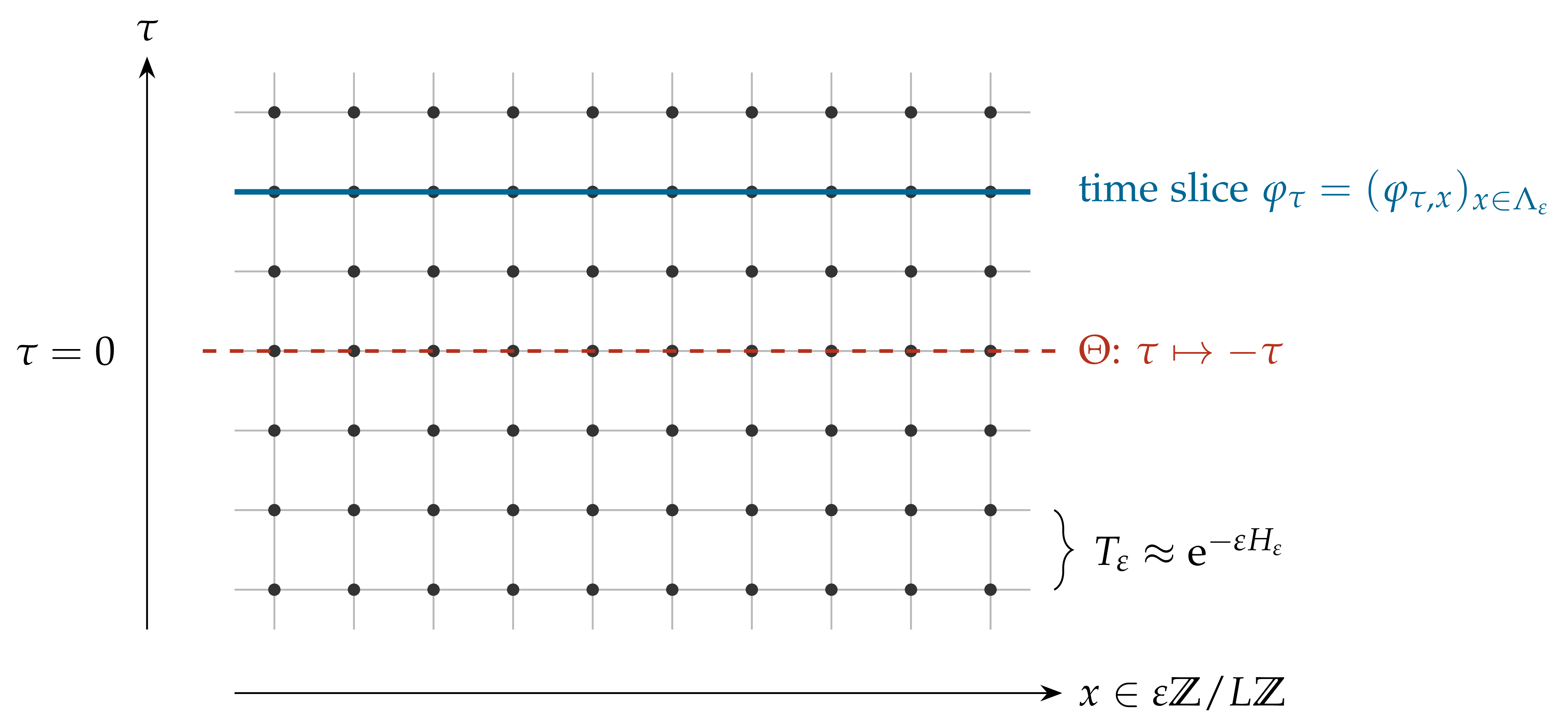
Fix \(L > 0\), \(N \in \mathbb{N}\), \(\varepsilon = L / N\), and the periodic lattice \(\Lambda_{\varepsilon} = \varepsilon \mathbb{Z}/ L\mathbb{Z} \subset \mathbb{T}_L\) (\(N\) sites). Configurations are \(\varphi = (\varphi_x)_{x \in \Lambda_{\varepsilon}} \in \mathbb{R}^{\Lambda_{\varepsilon}}\). In the Schrödinger representation \(\mathcal{H}_{\varepsilon} = L^2 (\mathbb{R}^{\Lambda_{\varepsilon}}, \mathrm{d} \varphi)\), \(\varphi_x\) acts by multiplication and \(\pi_x := - \mathrm{i} \varepsilon^{- 1} \partial / \partial \varphi_x\), so that \([\varphi_x, \pi_y] = \mathrm{i} \varepsilon^{- 1} \mathbb{1}_{x = y}\), the lattice version of \(\mathrm{i} \delta (x - y)\). Let \(V\) be a polynomial bounded below (e.g.

\(V (u) = \lambda u^4\)) and

where \((\nabla_{\varepsilon} \varphi)_x = (\varphi_{x + \varepsilon} - \varphi_x) / \varepsilon\) and \(U_{\varepsilon} (\varphi) = \varepsilon \sum_x [\frac{1}{2} (\nabla_{\varepsilon} \varphi)_x^2 + \frac{1}{2} m^2 \varphi_x^2 + V (\varphi_x)]\). A short computation (Exercise 2.1) shows that the Heisenberg fields \(\varphi_x (t) = \mathrm{e}^{\mathrm{i} tH_{\varepsilon}} \varphi_x \mathrm{e}^{- \mathrm{i} tH_{\varepsilon}}\) satisfy

a lattice regularisation of the quantum wave equation (1.9), now with a perfectly rigorous meaning.

\(H_{\varepsilon}\) is a Schrödinger operator on \(\mathbb{R}^N\) with a confining potential (\(U_{\varepsilon} \geq c| \varphi |^2 - C\) since \(m > 0\)). Hence it is essentially self-adjoint on \(C^{\infty}_c\), bounded below, with compact resolvent, and \(\mathrm{e}^{- tH_{\varepsilon}}\) is trace class for \(t > 0\). The integral kernel of \(\mathrm{e}^{- tH_{\varepsilon}}\) is strictly positive, so by the Perron–Frobenius argument the ground state energy \(E_0 = \inf \text{spec} H_{\varepsilon}\) is a simple eigenvalue with a strictly positive eigenfunction \(\Omega_{\varepsilon}\), the lattice vacuum [Sim79]. We set

2.2Positivity of the energy and analytic continuation

Let \(F_1, \ldots, F_n : \mathbb{R}^{\Lambda_{\varepsilon}} \to \mathbb{C}\) be bounded measurable (acting as multiplication operators) and \(F_j (t) = \mathrm{e}^{\mathrm{i} tH_{\varepsilon}} F_j \mathrm{e}^{- \mathrm{i} tH_{\varepsilon}}\). Since \(\bar{H} \Omega_{\varepsilon} = 0\),

Proposition 2.1. (Wick rotation) \(W\) depends only on \(\zeta_j = t_j - t_{j + 1}\) and extends to a function \(\mathcal{W} (\zeta_1, \ldots, \zeta_{n - 1})\) which is bounded and continuous on \(\bar{\mathbb{C}}_-^{\hspace{0.17em} n - 1}\) and analytic on \(\mathbb{C}_-^{n - 1}\), \(\mathbb{C}_- = \{ \text{Im} \zeta < 0\}\). At \(\zeta_j = - \mathrm{i} (\tau_j - \tau_{j + 1})\), \(\tau_1 \geq \ldots \geq \tau_n\), it gives the Schwinger functions

and the Schwinger functions determine the Wightman functions \(W\).

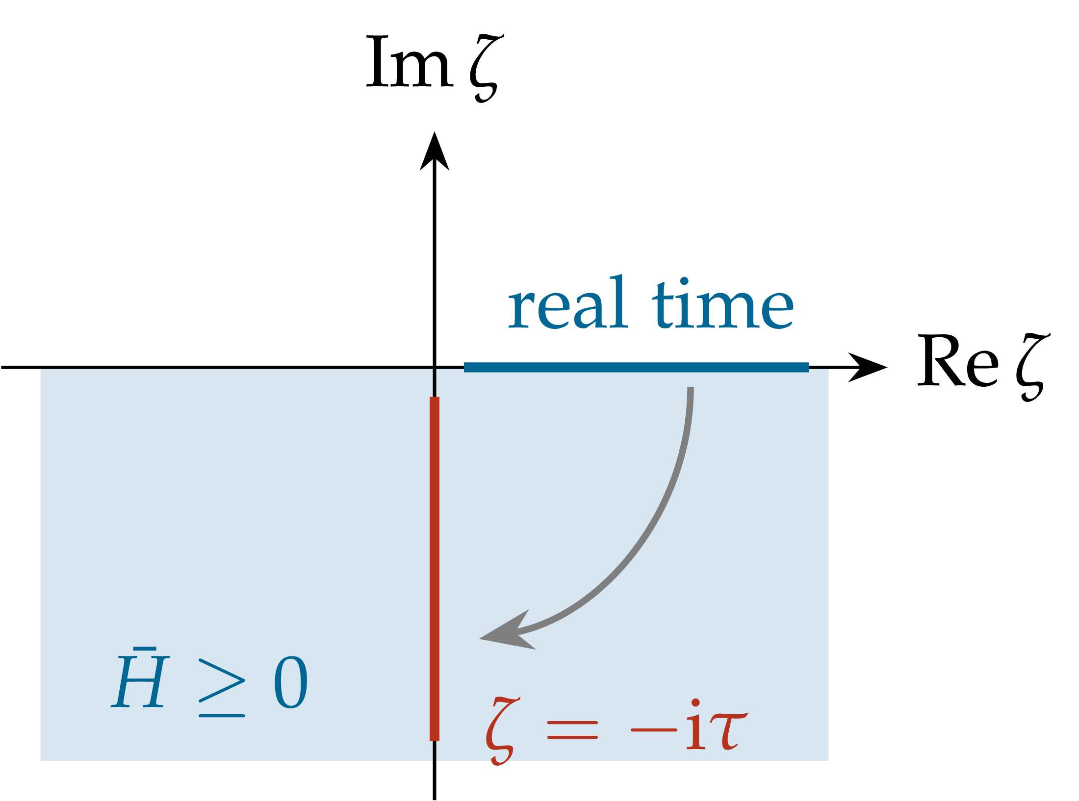
Proof. By the spectral theorem, \(\mathrm{e}^{- \mathrm{i} \zeta \bar{H}} = \int \mathrm{e}^{- \mathrm{i} \zeta \lambda} \mathrm{d} E (\lambda)\) with \(| \mathrm{e}^{- \mathrm{i} \zeta \lambda} | = \mathrm{e}^{\lambda \text{Im} \zeta} \leq 1\) for \(\lambda \geq 0\), \(\text{Im} \zeta \leq 0\). It is therefore a contraction, strongly continuous on \(\bar{\mathbb{C}}_-\) and analytic in the interior. Products of such operators give separately analytic, bounded, continuous functions, hence jointly analytic ones. If \(\mathcal{W}\) vanishes on \((- \mathrm{i} \mathbb{R}_+)^{n - 1}\), the identity theorem in \(\zeta_1\) (with the other variables on the imaginary axis) shows that it vanishes for all \(\zeta_1 \in \mathbb{C}_-\). Proceeding variable by variable, and using continuity up to the boundary, gives \(W \equiv 0\).\(\Box\)

Figure 2.1. Wick rotation (Proposition 2.1). Since \(\bar{H} \geq 0\), \(\mathrm{e}^{- \mathrm{i} \zeta \bar{H}}\) is a contraction on the lower half-plane \(\text{Im} \zeta \leq 0\), analytic in its interior. The Wightman functions on the real axis and the Schwinger functions on the negative imaginary axis are boundary values and restrictions of the same analytic function.

Remark 2.2. This is exactly where positivity of the energy enters: it allows rotating \(t \mapsto - \mathrm{i} \tau\) in all time differences simultaneously. It will be used twice more: \(\mathrm{e}^{- \tau \bar{H}}\), \(\tau \geq 0\), is a contraction semigroup, which can be represented as a path integral (Feynman–Kac); and \(\mathrm{e}^{- T \bar{H}}\) converges to the projection onto \(\ker \bar{H}\) as \(T \to \infty\), i.e. onto the vacuum when it is unique (Remark 2.7). (That the Feynman–Kac weights are positive is a separate fact, coming from the kinetic term.) In a relativistic theory, the Wightman functions are boundary values of functions analytic in the forward tube (Exercise 1.4). By Lorentz covariance and locality (the Bargmann–Hall–Wightman theorem and Jost points) these extend to a domain containing all non-coincident Euclidean points, where they define symmetric, Euclidean invariant Schwinger functions [SW64, OS73].

2.3Discretising imaginary time: the Feynman–Kac formula

The kinetic part of \(H_{\varepsilon}\) generates a Gaussian semigroup with kernel

Hence the symmetric Trotter approximant \(T_{\delta} := \mathrm{e}^{- \delta U_{\varepsilon} / 2} \hspace{0.17em} \mathrm{e}^{\frac{\delta}{2 \varepsilon} \Delta} \hspace{0.17em} \mathrm{e}^{- \delta U_{\varepsilon} / 2}\) has the explicit positive kernel

and \(T_{\delta}^{\lfloor \tau / \delta \rfloor} \to \mathrm{e}^{- \tau H_{\varepsilon}}\) strongly as \(\delta \to 0\) (Trotter product formula [RS80, Sim79]). Let \(T = J \delta\) and consider the space-time lattice

Writing the trace of a product of integral operators as an integral over closed chains, we get \(\text{Tr} (T_{\delta}^J) = (2 \pi \delta / \varepsilon)^{- NJ / 2} \int_{\mathbb{R}^{\Lambda}} \mathrm{e}^{- S_{\delta, \varepsilon} (\varphi)} \prod_{u \in \Lambda} \mathrm{d} \varphi_u\) with the lattice Euclidean action

This discretises \(S (\varphi) = \iint_{\mathbb{T}_T \times \mathbb{T}_L} [\frac{1}{2} (\partial_{\tau} \varphi)^2 + \frac{1}{2} (\partial_x \varphi)^2 + \frac{1}{2} m^2 \varphi^2 + V (\varphi)] \hspace{0.17em} \mathrm{d} \tau \hspace{0.17em} \mathrm{d} x\). Imaginary time and space now play symmetric roles: the Minkowski metric has become Euclidean. Define the probability measure

Inserting multiplication operators between the factors \(T_{\delta}\) gives, for \(\tau_1 \geq \ldots \geq \tau_n\) in \(\delta \mathbb{Z}\) with \(\tau_1 - \tau_n < T\),

where \(k_j = (\tau_j - \tau_{j + 1}) / \delta\) for \(j < n\) and \(k_n = J - \sum_{j < n} k_j\).

Proposition 2.3. (Feynman–Kac–Nelson) For bounded continuous \(F_j\) and dyadic \(\tau_1 \geq \ldots \geq \tau_n\),

Sketch. The Gaussian factor in (2.9) gives precisely the finite-dimensional distributions, at times \(\tau \in \delta \mathbb{Z}/ T\mathbb{Z}\), of the (unnormalised) Brownian loop measure on \(\mathbb{R}^{\Lambda_{\varepsilon}}\) of length \(T\) and generator \(\frac{1}{2 \varepsilon} \Delta\) (variance \(t / \varepsilon\) per coordinate). The potential term \(\delta \sum_{\tau} U_{\varepsilon} (\varphi_{\tau})\) is a Riemann sum for \(\int_0^T U_{\varepsilon} (\omega_{\tau}) \mathrm{d} \tau\). Hence, as \(\delta \to 0\) (along dyadic \(\delta\), say, so that the \(\tau_j\) stay on the lattice), both sides of (2.10) converge to the Feynman–Kac expression \(\text{Tr} (F_1 \mathrm{e}^{- (\tau_1 - \tau_2) H} \cdots F_n \mathrm{e}^{- (T - \tau_1 + \tau_n) H}) / \text{Tr} (\mathrm{e}^{- TH})\), written as an integral over Brownian loops weighted by \(\exp (- \int_0^T U_{\varepsilon})\) [Sim79]. The limit \(T \to \infty\) uses that \(E_0\) is simple and isolated (Exercise 2.6).\(\Box\)

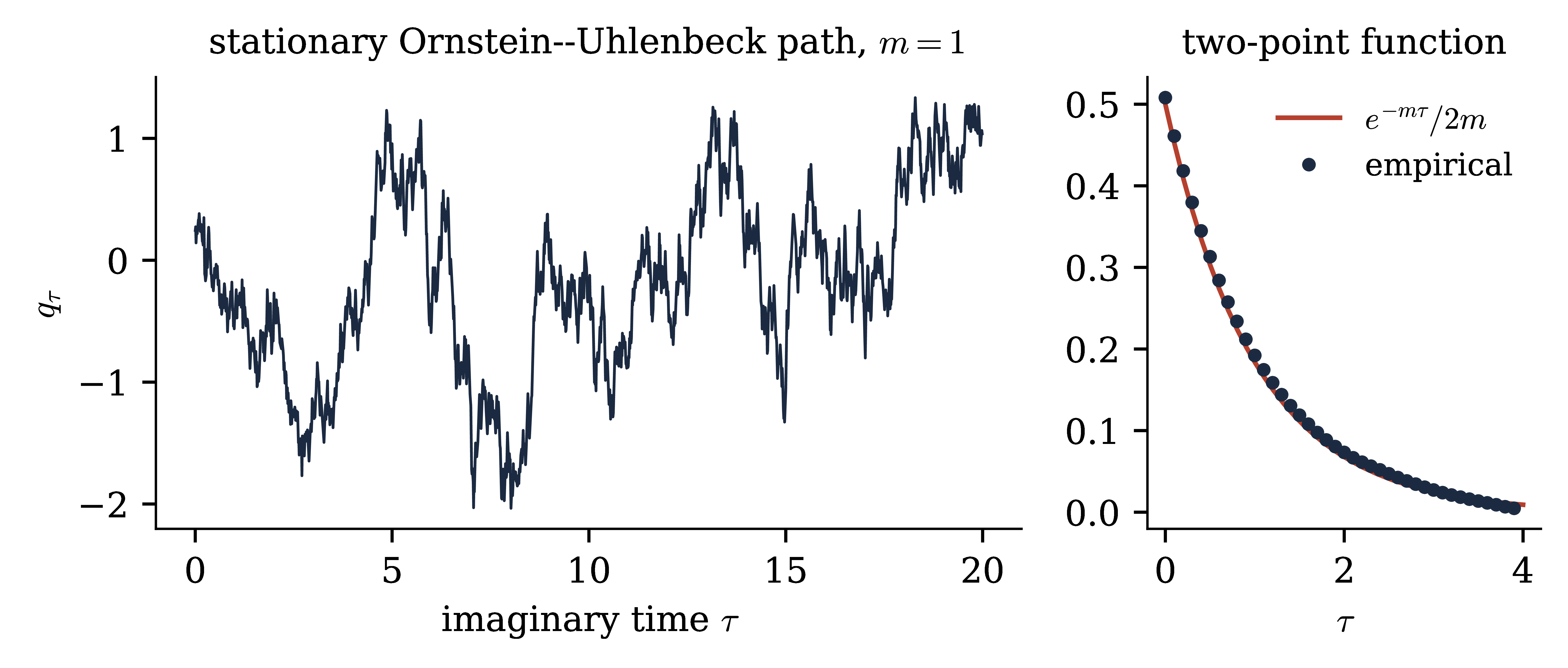
Vacuum expectations of the quantum system in imaginary time are thus moments of a classical probability measure. As \(T \to \infty\) the time-slices \((\varphi_{\tau})_{\tau \in \mathbb{R}}\) form a stationary Markov process: the ground-state transform of \(\mathrm{e}^{- \tau \bar{H}}\), whose one-time marginal is \(\Omega_{\varepsilon} (\varphi)^2 \mathrm{d} \varphi\). For \(N = 1\), \(V = 0\) this is the Ornstein–Uhlenbeck process (Exercise 2.2 and Figure 2.2).

Figure 2.2. Left: a sample of the stationary Ornstein–Uhlenbeck process, the imaginary-time path of one harmonic oscillator, i.e. the GFF in \(d = 1\) (Exercise 2.2). Right: its empirical two-point function against the Schwinger function \(\mathrm{e}^{- m \tau} / 2 m\).

2.4Classical statistical mechanics

Take the isotropic lattice \(\delta = \varepsilon\). Then (2.8) becomes

the first sum running over nearest-neighbour pairs of the two-dimensional periodic lattice \(\Lambda\). So \(\mu_{\varepsilon} \propto \prod_{\langle u, v \rangle} \mathrm{e}^{- \frac{1}{2} (\varphi_u - \varphi_v)^2} \prod_u \nu_{\varepsilon} (\mathrm{d} \varphi_u)\), with single-site measure \(\nu_{\varepsilon} (\mathrm{d} a) = \mathrm{e}^{- \varepsilon^2 (\frac{1}{2} m^2 a^2 + V (a))} \mathrm{d} a\). This is a ferromagnetic nearest-neighbour spin system with continuous, unbounded spins, i.e. a short-range model of classical statistical mechanics. In spacetime dimension \(d\) one gets \(\varepsilon^{d - 2} \sum_{\langle u, v \rangle}\) and \(\varepsilon^d \sum_u\) instead (Exercise 2.3). The nearest-neighbour structure makes \(\mu_{\varepsilon}\) reflection positive (Figure 2.3 and Exercise 2.5), the Euclidean shadow of the positivity of \(\mathrm{e}^{- \varepsilon H_{\varepsilon}}\). Conversely, reflection positivity is enough to reconstruct a Hilbert space and a positive Hamiltonian (Exercise 2.7).

Figure 2.3. The Euclidean space-time lattice. Rows are configurations of the quantum system at fixed imaginary time; the transfer matrix \(T_{\varepsilon} \approx \mathrm{e}^{- \varepsilon H_{\varepsilon}}\) connects consecutive rows. The nearest-neighbour structure makes the measure reflection positive with respect to \(\Theta\).

Remark 2.4. (Continuum limit \(=\) critical point) In lattice units the model (2.12) has mass \(\varepsilon m \to 0\), so its correlation length is \(\xi \approx (\varepsilon m)^{- 1} \to \infty\) lattice spacings (Exercise 2.4). The continuum limit of the regularised QFT is therefore the scaling limit of a family of short-range spin systems approaching a critical point. Conversely, any reflection positive, short-range critical model with a nontrivial scaling limit yields a candidate Euclidean QFT. This is Wilson's point of view on renormalisation [WK74]. For instance, the Griffiths–Simon construction realises \(\varphi^4\) single-spin measures as limits of normalised sums of ferromagnetically coupled Ising spins [GS73], and the critical 4D Ising and \(\varphi^4_4\) models have Gaussian scaling limits [ADC21]. See [GRS75] for the systematic use of lattice approximations for \(P (\varphi)_2\).

Remark 2.5. (Renormalisation already appears) For \(V (a) = \lambda a^4\), the limit \(\varepsilon \to 0\) at fixed \((m, \lambda)\) does not produce an interacting theory: the Gaussian part alone has \(c_{\varepsilon} := \mathbb{E} [\varphi_u^2] = \frac{1}{2 \pi} \log \frac{1}{\varepsilon m} + O (1)\) (compare (1.8)). One must take \(\varepsilon\)-dependent couplings, e.g. \(V_{\varepsilon} (a) = \lambda (a^4 - 6 c_{\varepsilon} a^2)\) (a divergent mass counterterm), i.e. \(\lambda\) times the Wick power \(: a^4\): of Section 3.3 up to a constant. In \(d = 2\) this is all that is needed; in \(d = 3\) more counterterms are required.

2.5Path integrals and the Osterwalder–Schrader axioms

Formally, as \(\varepsilon \to 0\) and \(L, T \to \infty\), (2.9) becomes the Euclidean path integral

Neither \(\mathcal{D} \varphi\) nor the action make sense, since typical \(\varphi\) are distributions. The Gaussian part, however, defines the Gaussian free field \(\mu_m\) of Section 3, and one is led to define \(\mu \propto \mathrm{e}^{- \int V (\varphi)} \mu_m\) with a renormalised \(V\), at least in finite volume in \(d = 2\). In \(d = 3\) this is possible only as the limit of ultraviolet-regularised measures of this form, and the limit is singular with respect to \(\mu_m\). Which measures on \(\mathcal{S}' (\mathbb{R}^d)\) correspond to relativistic QFTs? Let \(\hat{\mu} (f) := \int \mathrm{e}^{\mathrm{i} \varphi (f)} \mu (\mathrm{d} \varphi)\) be the characteristic functional and \(\Theta (\tau, \textbf{x}) = (- \tau, \textbf{x})\), \(\Theta f = f \circ \Theta\).

(OS0) Analyticity

For real \(f_1, \ldots, f_n \in C^{\infty}_c (\mathbb{R}^d)\), the map \(z \mapsto \hat{\mu} (\sum_j z_j f_j)\) is entire on \(\mathbb{C}^n\).

(OS1) Regularity

For some \(p \in [1, 2]\) and \(c > 0\), \(| \hat{\mu} (f) | \leq \exp (c (\|f\|_{L^1} +\|f\|_{L^p}^p))\) for all complex-valued \(f \in C^{\infty}_c (\mathbb{R}^d)\), with \(\hat{\mu}\) extended by (OS0); if \(p = 2\), the two-point function is in addition required to be locally integrable.

(OS2) Euclidean invariance

\(\hat{\mu} (f \circ g) = \hat{\mu} (f)\) for every Euclidean motion \(g\) of \(\mathbb{R}^d\).

(OS3) Reflection positivity

For real \(f_1, \ldots, f_n\) supported in \(\{\tau > 0\}\), the matrix \((\hat{\mu} (f_i - \Theta f_j))_{i, j}\) is positive semidefinite.

(OS4) Ergodicity

The time translations act ergodically on \((\mathcal{S}' (\mathbb{R}^d), \mu)\).

Theorem 2.6. (Osterwalder–Schrader reconstruction [OS73, OS75, GJ87]) If \(\mu\) satisfies (OS0)–(OS3), its moments are the Schwinger functions of a unique Wightman theory satisfying (W1)–(W4) and (W0) except possibly uniqueness of the vacuum. (OS4) holds iff the vacuum is unique.

Idea. Let \(\mathcal{E}_+\) be the functions of \(\varphi\) that depend only on its restriction to \(\{\tau > 0\}\), with \((F, G) := \mathbb{E}_{\mu} [\overline{\Theta F} \hspace{0.17em} G]\). By (OS3) this is a positive semi-definite form; quotienting by null vectors and completing gives \(\mathcal{H}\). Time translations by \(t \geq 0\) map \(\mathcal{E}_+\) to itself and descend to a self-adjoint contraction semigroup \(\mathrm{e}^{- tH}\), so \(H \geq 0\): positivity of the energy is recovered from reflection positivity. The vacuum is the class of \(1\), and the analytic continuation \(\tau \to \mathrm{i} t\) yields the Wightman functions.\(\Box\)

Remark 2.7. (Positivity, clustering and uniqueness of the vacuum) Let \(H \geq 0\) be self-adjoint, \(\Omega \in \ker H\), and let \(P_0\) be the orthogonal projection onto \(\ker H\). Positivity of the energy turns uniqueness of the vacuum into a clustering statement, in three steps.

(i) Imaginary time: no averaging is needed. By the spectral theorem and dominated convergence, \(\mathrm{e}^{- tH} = \int_{[0, \infty)} \mathrm{e}^{- t \lambda} \mathrm{d} E (\lambda) \to E (\{0\}) = P_0\) strongly as \(t \to \infty\), because \(\mathrm{e}^{- t \lambda} \to \mathbb{1}_{\lambda = 0}\) for \(\lambda \geq 0\). In the reconstruction above, for \(F, G \in \mathcal{E}_+\) and \(\tau_t\) the time translation,

So the Euclidean correlations cluster, \(\mathbb{E}_{\mu} [\overline{\Theta F} \hspace{0.17em} \tau_t G] \to \overline{\mathbb{E}_{\mu} F} \hspace{0.17em} \mathbb{E}_{\mu} G\), iff \(P_0\) is the projection onto \(\mathbb{C} \Omega\), i.e. iff the vacuum is unique. With a mass gap the convergence is exponential, at rate \(\inf (\text{spec} H \setminus \{0\})\) (Exercise 2.6). Moreover, the spectrum condition \(H \geq | \textbf{P} |\) implies that a vector with \(H \psi = 0\) also has \(\textbf{P} \psi = 0\): invariance under time translations already gives invariance under all translations. For reflection positive measures, ergodicity (OS4) (by the reconstruction theorem) and clustering in imaginary time (by (i)) are both equivalent to uniqueness of the vacuum.

(ii) Real time: only averages converge. The unitary group \(\mathrm{e}^{- \mathrm{i} tH}\) does not converge as \(t \to \infty\) in general. Only its time averages do: \(\frac{1}{T} \int_0^T \mathrm{e}^{- \mathrm{i} tH} \mathrm{d} t \to P_0\) strongly (von Neumann's mean ergodic theorem). If \(H\) has an eigenvalue \(E > 0\) with eigenvector \(\psi\), then \(\langle \psi, \mathrm{e}^{- \mathrm{i} tH} \psi \rangle = \mathrm{e}^{- \mathrm{i} tE} \| \psi \|^2\) oscillates forever, while \(\langle \psi, \mathrm{e}^{- tH} \psi \rangle = \mathrm{e}^{- tE} \| \psi \|^2 \to 0\). This is the situation of the lattice systems of Section 2 in finite volume: their real-time correlations never decay, although the vacuum is unique and the Euclidean correlations cluster exponentially.

(iii) Relativistic theories. Here Lorentz covariance removes the eigenvalues. If \(U (a, \mathbb{1}) \psi = \mathrm{e}^{\mathrm{i} p \cdot a} \psi\) with \(p \neq 0\), then \(U (0, \Lambda) \psi\) is an eigenvector with eigenvalue \(\Lambda p\). The orbit of \(p\) is uncountable and eigenvectors for distinct eigenvalues are orthogonal, which contradicts the separability of \(\mathcal{H}\). So, if the vacuum is unique, the spectral measures of the translations on \(\Omega^{\perp}\) have no atoms, and by Wiener's theorem correlations cluster in mean:

Locality then upgrades this to the pointwise cluster property (e) in spacelike directions [SW64]. With a mass gap, the truncated functions decay faster than any power (Ruelle [Rue62]), and in fact exponentially (Araki, Hepp and Ruelle [AHR62]); see [Haa96, §II.4]. Conversely, if \(\ker H\) contains a unit vector \(\psi \perp \Omega\), then by cyclicity (W4) some product of fields has a nonzero component along \(\psi\), and the corresponding correlations do not factorise. In Euclidean terms the measure is then a mixture of several ergodic components, or phases, as for \(\varphi^4_2\) at strong coupling with its symmetric mixture of the two pure phases [GJS75].

The Euclidean strategy.

Exercises

3The course

These notes cover the first of six two-hour lectures given at SISSA, Trieste, in October–November 2026, for graduate students in analysis, probability or mathematical physics. Lectures 1–3 have their own notes; the content of Lectures 4–6 is not yet settled. They will probably be devoted to a construction of \(\Phi^4_3\) on the torus via the FBSDE of Lecture 3.

Prerequisites.

Approach.

Lecture 1. Relativistic quantum fields and imaginary time

Lecture 2. The Gaussian free field

Lecture 3. Stochastic observables, the Polchinski flow and FBSDEs

Homework and projects.

References and further reading

Guide.

[ADC21]

M. Aizenman, H. Duminil-Copin. Marginal triviality of the scaling limits of critical 4D Ising and \(\phi^4_4\) models. Ann. of Math. 194 (2021), 163–235.

[ADG20]

S. Albeverio, F.C. De Vecchi, M. Gubinelli. Elliptic stochastic quantization. Ann. Probab. 48 (2020), 1693–1741.

[AHR62]

H. Araki, K. Hepp, D. Ruelle. On the asymptotic behaviour of Wightman functions in space-like directions. Helv. Phys. Acta 35 (1962), 164–174.

[BBD24]

R. Bauerschmidt, T. Bodineau, B. Dagallier. Stochastic dynamics and the Polchinski equation: an introduction. Probab. Surveys 21 (2024).

[BBS19]

R. Bauerschmidt, D.C. Brydges, G. Slade. Introduction to a Renormalisation Group Method. Lecture Notes in Math. 2242, Springer, 2019.

[BCG26]

I. Bailleul, I. Chevyrev, M. Gubinelli. Stochastic observables and Wilson–Itô diffusions. In preparation.

[BD98]

M. Boué, P. Dupuis. A variational representation for certain functionals of Brownian motion. Ann. Probab. 26 (1998), 1641–1659.

[BFV03]

R. Brunetti, K. Fredenhagen, R. Verch. The generally covariant locality principle: a new paradigm for local quantum field theory. Comm. Math. Phys. 237 (2003), 31–68.

[BG20]

N. Barashkov, M. Gubinelli. A variational method for \(\Phi^4_3\). Duke Math. J. 169 (2020), 3339–3415.

[Bry09]

D.C. Brydges. Lectures on the renormalisation group. In Statistical Mechanics, IAS/Park City Math. Ser. 16, Amer. Math. Soc., 2009, 7–93.

[BSZ92]

J.C. Baez, I.E. Segal, Z. Zhou. Introduction to Algebraic and Constructive Quantum Field Theory. Princeton Series in Physics, Princeton University Press, 1992.

[DPZ14]

G. Da Prato, J. Zabczyk. Stochastic Equations in Infinite Dimensions, 2nd ed. Cambridge University Press, 2014.

[FH81]

K. Fredenhagen, J. Hertel. Local algebras of observables and pointlike localized fields. Comm. Math. Phys. 80 (1981), 555–561.

[FO76]

J. Feldman, K. Osterwalder. The Wightman axioms and the mass gap for weakly coupled \((\Phi^4)_3\) quantum field theories. Ann. Physics 97 (1976), 80–135.

[GJ68]

J. Glimm, A. Jaffe. A \(\lambda \varphi^4\) quantum field theory without cutoffs. I. Phys. Rev. 176 (1968), 1945–1951.

[GJ73]

J. Glimm, A. Jaffe. Positivity of the \(\varphi^4_3\) Hamiltonian. Fortschr. Phys. 21 (1973), 327–376.

[GJ87]

J. Glimm, A. Jaffe. Quantum Physics: A Functional Integral Point of View, 2nd ed. Springer, 1987.

[GJS74]

J. Glimm, A. Jaffe, T. Spencer. The Wightman axioms and particle structure in the \(P (\varphi)_2\) quantum field model. Ann. of Math. 100 (1974), 585–632.

[GJS75]

J. Glimm, A. Jaffe, T. Spencer. Phase transitions for \(\varphi^4_2\) quantum fields. Comm. Math. Phys. 45 (1975), 203–216.

[GRS75]

F. Guerra, L. Rosen, B. Simon. The \(P (\varphi)_2\) Euclidean quantum field theory as classical statistical mechanics. I, II. Ann. of Math. 101 (1975), 111–189 and 191–259.

[GS73]

R.B. Griffiths, B. Simon. The \((\varphi^4)_2\) field theory as a classical Ising model. Comm. Math. Phys. 33 (1973), 145–164.

[Haa96]

R. Haag. Local Quantum Physics, 2nd ed. Springer, 1996.

[HK64]

R. Haag, D. Kastler. An algebraic approach to quantum field theory. J. Math. Phys. 5 (1964), 848–861.

[Jaf00]

A. Jaffe. Constructive quantum field theory. In Mathematical Physics 2000, Imperial College Press, 2000, 111–127.

[Jan97]

S. Janson. Gaussian Hilbert Spaces. Cambridge University Press, 1997.

[Kal52]

G. Källén. On the definition of the renormalization constants in quantum electrodynamics. Helv. Phys. Acta 25 (1952), 417.

[KLP84]

A. Klein, L.J. Landau, J.F. Perez. Supersymmetry and the Parisi–Sourlas dimensional reduction: a rigorous proof. Comm. Math. Phys. 94 (1984), 459–482.

[Leh54]

H. Lehmann. Über Eigenschaften von Ausbreitungsfunktionen und Renormierungskonstanten quantisierter Felder. Nuovo Cimento 11 (1954), 342–357.

[Nel66]

E. Nelson. A quartic interaction in two dimensions. In Mathematical Theory of Elementary Particles, MIT Press, 1966, 69–73.

[Nel73a]

E. Nelson. The free Markoff field. J. Funct. Anal. 12 (1973), 211–227.

[Nel73b]

E. Nelson. Construction of quantum fields from Markoff fields. J. Funct. Anal. 12 (1973), 97–112.

[OS73]

K. Osterwalder, R. Schrader. Axioms for Euclidean Green's functions. Comm. Math. Phys. 31 (1973), 83–112.

[OS75]

K. Osterwalder, R. Schrader. Axioms for Euclidean Green's functions II. Comm. Math. Phys. 42 (1975), 281–305.

[Pol84]

J. Polchinski. Renormalization and effective Lagrangians. Nuclear Phys. B 231 (1984), 269–295.

[Rad96]

M.J. Radzikowski. Micro-local approach to the Hadamard condition in quantum field theory on curved space-time. Comm. Math. Phys. 179 (1996), 529–553.

[RS75]

M. Reed, B. Simon. Methods of Modern Mathematical Physics II: Fourier Analysis, Self-Adjointness. Academic Press, 1975.

[RS80]

M. Reed, B. Simon. Methods of Modern Mathematical Physics I: Functional Analysis, rev. ed. Academic Press, 1980.

[Rue62]

D. Ruelle. On the asymptotic condition in quantum field theory. Helv. Phys. Acta 35 (1962), 147–163.

[Seg70]

I.E. Segal. Construction of non-linear local quantum processes: I. Ann. of Math. 92 (1970), 462–481.

[She07]

S. Sheffield. Gaussian free fields for mathematicians. Probab. Theory Related Fields 139 (2007), 521–541.

[Sim74]

B. Simon. The \(P (\varphi)_2\) Euclidean (Quantum) Field Theory. Princeton University Press, 1974.

[Sim79]

B. Simon. Functional Integration and Quantum Physics. Academic Press, 1979; 2nd ed., AMS Chelsea, 2005.

[Sum12]

S.J. Summers. A perspective on constructive quantum field theory. Preprint, arXiv:1203.3991.

[SW64]

R.F. Streater, A.S. Wightman. PCT, Spin and Statistics, and All That. Benjamin, 1964; Princeton Landmarks in Physics, 2000.

[Sym69]

K. Symanzik. Euclidean quantum field theory. In Local Quantum Theory (R. Jost, ed.), Proc. Int. School of Physics “Enrico Fermi” 45, Academic Press, 1969.

[Wal94]

R.M. Wald. Quantum Field Theory in Curved Spacetime and Black Hole Thermodynamics. University of Chicago Press, 1994.

[Wig64]

A.S. Wightman. La théorie quantique locale et la théorie quantique des champs. Ann. Inst. H. Poincaré Sect. A 1 (1964), 403–420.

[WK74]

K.G. Wilson, J. Kogut. The renormalization group and the \(\epsilon\) expansion. Phys. Rep. 12 (1974), 75–199.