Constructive quantum field theory — Lecture 2 (slides)
A Constructive Introduction to Quantum
Field Theory
The Gaussian free field
Massimiliano Gubinelli | University of Oxford
SISSA lectures, Lecture 2 — notes:
Lecture 2, §3
Where we are
Last time. Positivity of the energy \(\Rightarrow\)
imaginary time; vacuum expectations are moments of \(\mu
(\mathrm{d} \varphi) \hspace{0.17em} \backprime\backprime =
"
\hspace{0.17em} Z^{- 1} \mathrm{e}^{- \int [\frac{1}{2} | \nabla
\varphi |^2 +
\frac{1}{2} m^2 \varphi^2 + V (\varphi)]} \mathcal{D}
\varphi\); relativistic QFTs \(\leftrightarrow\)
measures on \(\mathcal{S}' (\mathbb{R}^d)\)
satisfying the OS axioms.
Today. The Gaussian part, rigorously.
Construction on \(\mathbb{T}^d\) and \(\mathbb{R}^d\); regularity.
Reflection positivity; the free field;
Källén–Lehmann again.
Local operators: Wick powers.
Gaussian integration by parts: the Dyson–Schwinger (DS)
equation.
DS characterises the GFF.
Definition and
construction
Lecture 2
Setting and definition
\(\mathcal{M}=\mathbb{T}^d_L = (\mathbb{R}/
L\mathbb{Z})^d\) or \(\mathbb{R}^d\);\(\mathcal{S} (\mathcal{M})\)
smooth, resp. Schwartz, functions;\(\mathcal{S}'
(\mathcal{M})\) with the cylinder (\(=\)
Borel) \(\sigma\)-algebra.
\(\displaystyle A := m^2 - \Delta, \qquad C := A^{- 1}, \qquad m >
0.\)
\(A\), \(C\) are continuous
bijections of \(\mathcal{S} (\mathcal{M})\)
(Fourier multipliers \((|k|^2 + m^2)^{\pm 1}\)),
and \(\|C\|_{L^2 \to L^2} \leqslant m^{- 2}\).
Definition.
The Gaussian free field\(\mu_m\) is the centred Gaussian measure on
\(\mathcal{S}' (\mathcal{M})\) with
Formally \(\mu_m (\mathrm{d} \varphi)
\backprime\backprime = "Z^{- 1} \mathrm{e}^{-
\frac{1}{2} \langle
\varphi, A \varphi \rangle} \mathcal{D} \varphi\): the Gaussian
part of the Euclidean action.
Decay \(\approx \mathrm{e}^{- m |x|}\) at
infinity.
Singular on the diagonal for \(d \geqslant
2\): the field is not a function.
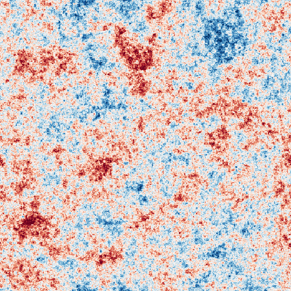
A sample of the massive GFF
on \(\mathbb{T}^2\) (\(m =
4\), \(512^2\) Fourier modes).
Existence on the torus
Theorem.
Let \((e_n)\) be a
real orthonormal basis of eigenfunctions of \(-
\Delta\) on \(\mathbb{T}^d_L\), \(- \Delta e_n = \kappa_n e_n\), \(\lambda_n
= m^2 + \kappa_n\), and \((g_n)\) i.i.d.
\(N (0, 1)\). For \(s > \frac{d}{2}
- 1\),
\(L^2\)-bounded \(H^{-
s}\)-valued martingale \(\Rightarrow\)
convergence. And \(\varphi (f) = \sum_n \lambda_n^{- 1 /
2} g_n \langle e_n, f \rangle\) is Gaussian with variance
\(\sum_n \lambda_n^{- 1} \langle e_n, f \rangle^2 =
\langle f, Cf \rangle\).
Existence on \(\mathbb{R}^d\) and regularity
Bochner–Minlos
\(\Psi : \mathcal{S} (\mathbb{R}^d) \to
\mathbb{C}\) continuous, positive definite, \(\Psi
(0) = 1\)\(\Rightarrow\) there is a
unique probability measure on \(\mathcal{S}'
(\mathbb{R}^d)\) with characteristic functional \(\Psi\).
For \(\Psi (f) = \mathrm{e}^{- \frac{1}{2} \langle f, Cf
\rangle}\): continuity from \(\langle f, Cf
\rangle \leqslant m^{- 2} \|f\|_{L^2}^2\); positive
definiteness from \(\Psi (f_j - f_k) = a_j a_k
\mathrm{e}^{\langle f_j, Cf_k \rangle}\) and the Schur product
theorem.
Regularity (sharp, Exercise 3.3):
\(d = 1\)
\(d = 2\)
\(d = 3\)
stationary OU process
\(H^{- \kappa}\), \(\forall
\kappa > 0\); not a function
\(H^{- 1 / 2 - \kappa}\)
The Cameron–Martin space \(H^1\) (finite
action) has measure zero.
OS reconstruction of \(\mu_m\) gives the
free field of mass \(m\):
Fock space over \(L^2 (N)\), \(H
= \mathrm{d} \Gamma (\omega)\) (Nelson's free Markov
field).
The time-zero field\(\varphi (0,
\cdot)\) exists and is Gaussian with covariance \((2 \omega)^{- 1}\): the ground state measure \(\Omega_0^2 \mathcal{D} \varphi\) of the free
Hamiltonian in the Schrödinger representation.
The GFF is the continuum limit of the lattice spin system of
Lecture 1 with \(V = 0\) (Exercise 3.10).
Markov property (Nelson): rooted in the locality of \(A\).
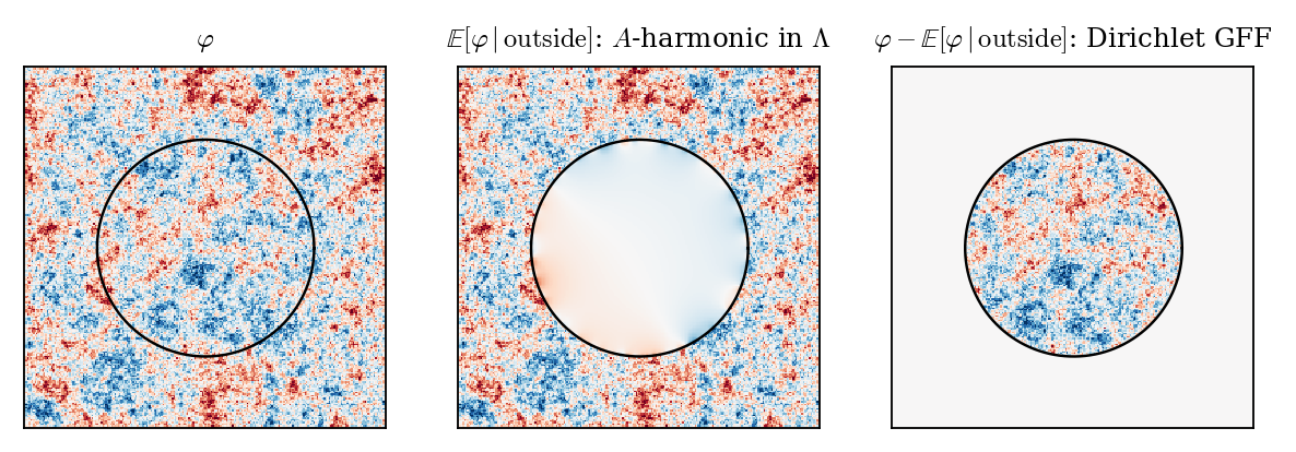
Nelson's Markov property
Markov for \(\Lambda\):
inside and outside are conditionally independent given the field
near \(\partial \Lambda\).
The GFF is Markov for every open \(\Lambda\)
(Nelson 1973): \(\mathbb{E} [\varphi (f)
\hspace{0.17em} | \hspace{0.17em} \text{outside}] =
\varphi (\Pi
f)\), and \(\Pi f = Au\) is supported
on \(\partial \Lambda\)because \(A = m^2 - \Delta\) is local. Given the
outside: harmonic extension \(+\) independent
Dirichlet GFF (next slide).
Markov \(+\) sharp \(\Sigma_0\)\(\Rightarrow\) RP: with \(\Sigma_0\)
the time-zero field, \(\mu\)\(\Theta\)-invariant,
\(\Theta\) trivial on \(\Sigma_0\):
Nelson's reconstruction (1973), before Osterwalder–Schrader.
Relevance: preserved by local perturbations \(\mathrm{e}^{- \int_{\Lambda} V}\)\(\Rightarrow\)\(P (\varphi)_2\) as classical statistical
mechanics (Guerra–Rosen–Simon). Not stable under
limits; OS use RP instead: not comparable (generalised free fields
are RP, not Markov; the \(P^{- 1}\) field is
Markov, not RP), but closed under weak limits.
\(\displaystyle \varphi = h + \psi, \qquad (m^2 - \Delta) h = 0
\text{in } \Lambda, \quad h =
\varphi \text{on } \partial \Lambda,\)
\(h =\mathbb{E} [\varphi \hspace{0.17em} |
\hspace{0.17em} \text{outside}]\) depends only on the field
at the boundary; \(\psi\) is a
Dirichlet GFF, independent of the outside.
Symanzik: fields and Brownian paths
Symanzik (1966, 1969): QFT through Schwinger functions as moments
of a classical Markov field — the Euclidean programme.
Paths:\(C (x, y) = \int_0^{\infty}
\mathrm{e}^{- m^2 t} p_t (x, y) \hspace{0.17em}
\mathrm{d}
t\) is the Green function of a killed Brownian motion. For
\(\mathrm{e}^{- \int V} \mu_m\): a gas of
paths and loops interacting through local times; for \(\varphi^4\),
intersections are penalised (lattice:
Brydges–Fröhlich–Spencer 1982; triviality for
\(d > 4\)).
Loop soups (Lawler–Werner 2004): Poisson
cloud of Brownian loops of intensity \(\alpha\);
on a graph \(\mathbb{E} \hspace{0.17em} \mathrm{e}^{-
\langle \chi, L \rangle} = \det (1 +
C \chi)^{- \alpha}\).
Le Jan's isomorphism: for \(\alpha =
\frac{1}{2}\) the occupation field is \(\frac{1}{2}
\varphi^2\); in \(d = 2, 3\) the
renormalised one is \(\frac{1}{2} :
\varphi^2\):.
Lupu 2016: loop clusters \(=\) sign clusters
of the cable-graph GFF. Werner 2016: spatial Markov property of
loop soups. Qian–Werner 2019. Survey: Werner–Powell.
Euclidean Källén–Lehmann
Wick rotation of \(W_2^{(M)}\): \(\int
\mathrm{d} \Omega_M (\textbf{p}) \hspace{0.17em} \mathrm{e}^{-
\omega_M
(\textbf{p}) | \tau | + \mathrm{i} \textbf{p} \cdot
\textbf{x}} = G_M (\tau,
\textbf{x})\). Hence for any theory
satisfying the axioms
Short distances.\(G_M\)
decreases in \(M\) and \(G_M /
G_m \to 1\) at \(0\) (\(d
\geqslant 2\)), so \(\liminf_{x \to 0} S_2^T
(x) / G_m (x) \geqslant \rho ([0, \infty)) > 0\): never
less singular than free. Scale invariance \(\Rightarrow\)
unitarity bound \(\Delta \geqslant \frac{d -
2}{2}\) (Exercise 3.2).
Long distances.\(\text{supp} \rho
\subset [m_0^2, \infty)\)\(\Leftrightarrow\)
decay at least like \(\mathrm{e}^{- m_0
|x|}\): mass gap \(=\) clustering.
Two masses: a positive but nonlocal theory
\(\rho = c_1^2 \delta_{m_1^2} + c_2^2
\delta_{m_2^2}\), \(0 < m_1 < m_2\):\(C_{\rho} = c_1^2 (m_1^2 - \Delta)^{- 1}
+ c_2^2 (m_2^2 - \Delta)^{- 1}\), the law of \(c_1
\varphi_1 + c_2 \varphi_2\) (independent GFFs). RP for each
term \(\Rightarrow\) OS axioms.
It reconstructs to two free species
\(\mathcal{H}= \Gamma (\mathfrak{h}_{m_1}) \otimes
\Gamma (\mathfrak{h}_{m_2})\),\(\varphi = c_1 \varphi_{m_1} \otimes \mathbb{1} + c_2
\hspace{0.17em}
\mathbb{1} \otimes \varphi_{m_2}\),\(W_2 = c_1^2 W_2^{(m_1)} + c_2^2
W_2^{(m_2)}\). Two kinds of free particles, created by
the same field; no scattering (truncated \(W_{n
\geqslant 3} = 0\)).
What is lost:
\((\Box + m_1^2) (\Box + m_2^2) \varphi =
0\), but no Klein–Gordon equation; \((\varphi
(0), \pi (0))\) are not complete Cauchy data.
so \(\rho = (\delta_{m_1^2} - \delta_{m_2^2}) / (m_2^2 -
m_1^2)\) has a negative weight.
By Euclidean Källén–Lehmann it is not
reflection positive: the mass \(m_2\)
is a ghost of negative norm (Pais–Uhlenbeck,
Lee–Wick).
Same for any \(1 / \hat{C} =\) polynomial of
degree \(\geqslant 2\): \(s
\hspace{0.17em} \hat{C} (s) \to 0\), while \(s
\int \frac{\rho (\mathrm{d} M^2)}{s + M^2} \uparrow \rho ([0,
\infty))\).
Moral
For Gaussian fields, positivity (OS) and locality
of the Euclidean field equation (\(C^{- 1}\) a
differential operator) together single out the free field:
covariance \(c (m^2 - \Delta)^{- 1}\) (or white
noise).
Is the nonlocal theory physical?
In Minkowski space, yes: all Wightman axioms
hold, including locality (W3); positive energy, unique vacuum. Two
free species: trivial and redundant, not inconsistent.
“Nonlocal” is Euclidean: no Markov
property \(\Leftrightarrow\)\(\varphi\)
alone is not a complete set of local degrees of freedom (no Cauchy
problem, no Lagrangian in \(\varphi\) only).
Cure: the pair \((\varphi_1, \varphi_2)\) is
local and Markov.
Continuous \(\rho\) (a
continuum of free species) is unphysical: no dynamical law of
finite order, and too many localised states.
Buchholz–Wichmann nuclearity (cf. Haag–Swieca) needs
\(\sum_i n_i \mathrm{e}^{- \beta m_i} <
\infty\): no sensible thermodynamics.
Interacting theories also have a continuum in
\(\rho\), but produced by a local
interaction: the Euclidean field equation of \(\Phi^4_2\),
with \((m^2 - \Delta) \varphi + 4 \lambda :
\varphi^3\): in the DS equation, is local.
Local operators: Wick
products
Lecture 2
Hermite polynomials
Interactions \(\int V (\varphi (x)) \mathrm{d} x\)
need local functions of \(\varphi (x)\):
regularise, subtract, remove the regularisation.
Renormalisation:\(\varphi_{\varepsilon}
(x)^n\) has no limit; subtracting \(c_{\varepsilon}
\to \infty\) (via \(H_n\)) is the
simplest counterterm. A different mollifier changes \(:
\varphi^n\): by lower Wick powers with finite
coefficients (Exercise 3.4).
Chaos:\(: \varphi^n : (f)\)
lies in the \(n\)-th Wiener chaos; \(L^2 (\mu_m) \simeq\) Fock space over \(H^{-
1} (\mathcal{M})\). Hypercontractivity \(\|X\|_{L^p}
\leqslant (p - 1)^{n / 2} \|X\|_{L^2}\) gives convergence
in all \(L^p\) (and in \(\mathcal{C}^{-
\kappa}\) for \(d = 2\)).
Towards \(\Phi^4_2\): on
\(\mathbb{T}^2\), \(\int :
\varphi^4 : \in \bigcap_p L^p\) and (Nelson) \(\mathrm{e}^{-
\lambda \int : \varphi^4 :} \in L^1 (\mu_m)\).
Other local operators:\(\partial^{\alpha}
\varphi\); in \(d = 2\) the Wick
exponentials \(: \mathrm{e}^{\mathrm{i} \beta
\varphi}\):, in \(L^2\) iff \(\beta^2 < 4 \pi\) (sine-Gordon; Exercise 3.6).
The Dyson–Schwinger
equation
Lecture 2
Beyond \(L^2\): Wick powers do not exist
If \(n (d - 2) \geqslant d\): \(\mathbb{E}
[: \varphi_{\varepsilon}^n : (f)^2] \to \infty\). Worse:
there is no random distribution at all, in any
topology or on any space. Albeverio–Liang 2007: \(:
\varphi^2 : (f)\), \(f > 0\), in \(d = 4\) (and \(d \geqslant
5\)) is a Hida distribution, not a random variable.
Bounded chaos: the law is controlled by \(\sigma
= \|X\|_2\). Upper tails \(\|X\|_p
\leqslant (p - 1)^{n / 2} \sigma\) (hypercontractivity);
\(\mathbb{P} (|X| > \frac{1}{2} \sigma) \geqslant
c_n\) (Paley–Zygmund); \(\mathbb{P} (|X|
\leqslant t \sigma) \leqslant Cnt^{1 / n}\)
(Carbery–Wright). So: tight \(\Leftrightarrow\)
bounded in \(L^2\); in probability \(\Leftrightarrow\) in \(L^2\).
Renormalising by \(\sigma_{\varepsilon}^{-
1}\) typically gives Gaussian limits (fourth moment
theorem; Albeverio–Zhou 1996): the \(n\)-th
power is lost.
Gaussian integration by parts
Cylinder functions \(\mathcal{F}C^{\infty}_b \ni F
(\varphi) = g (\varphi (f_1), \ldots, \varphi
(f_n))\), \(g \in C^{\infty}_b\):
\(\displaystyle D_h F (\varphi) = \left. \frac{\mathrm{d}}{\mathrm{d}
t} F (\varphi + th)
\right|_{t = 0} = \sum_i \partial_i g (\ldots)
\langle f_i, h \rangle =
\langle DF, h \rangle, \qquad DF (x) =
\frac{\delta F}{\delta \varphi (x)} .\)
Lemma.
\((Y, X_1, \ldots,
X_n)\) centred Gaussian:\(\mathbb{E}
[Y \hspace{0.17em} g (X)] = \sum_i \mathbb{E} [YX_i]
\hspace{0.17em} \mathbb{E} [\partial_i g (X)]\).
Proof. For \(g = \mathrm{e}^{\mathrm{i} \langle u,
\cdot \rangle}\): \(\mathbb{E} [Y
\mathrm{e}^{\mathrm{i} \langle u, X \rangle}] = -
\mathrm{i}
\partial_{\theta} \mathbb{E}[\mathrm{e}^{\mathrm{i} \theta
Y + \mathrm{i}
\langle u, X \rangle}] |_{\theta = 0} = \mathrm{i}
\sum_i u_i \mathbb{E}
[YX_i] \mathbb{E} [\mathrm{e}^{\mathrm{i}
\langle u, X \rangle}]\); then Fourier inversion and
approximation.
The Dyson–Schwinger equation
Proposition.
For all \(F \in
\mathcal{F}C^{\infty}_b\), \(h \in \mathcal{S}
(\mathcal{M})\):
the Euclidean version of \((\Box + m^2) \varphi + V'
(\varphi) = 0\).
\(V' (\varphi)\) must be a well-defined local
operator: \(\Phi^4_2\): \(V' = 4
\lambda : \varphi^3\):; field equation for \(P
(\varphi)_2\): Dimock–Glimm 1974,
Albeverio–Röckner 1991. For \(\Phi^4_3\)
the renormalised field equation goes back to
Feldman–Rączka 1977; renormalised cubic term as a
random distribution: Gubinelli–Hofmanová 2021.
Defining \(V' (\varphi)\): point splitting and the
OPE
\(\varphi^3 (x)\): product at one point.
Point splitting: regular part of \(\varphi
(y_1) \varphi (y_2) \varphi (y_3)\) as \(y_i
\to x\).
OPE (Wilson 1969, Zimmermann 1973): products at
nearby points \(=\) local operators \(\times\) singular coefficients; composite operator
\(=\) regular part. Field equation \((\Box + m^2) \varphi = - 4 \lambda N
[\varphi^3]\).
The coefficients are those of the interacting
theory. \(\Phi^4_2\): Gaussian subtraction
suffices (Schrader 1974). \(\Phi^4_3\): an
extra \(\delta_{\varepsilon}
\varphi_{\varepsilon}\), \(\delta_{\varepsilon}
\sim \lambda \log (1 / \varepsilon)\): \(4
\lambda \delta_{\varepsilon}\) is the sunset mass
counterterm (Gubinelli–Hofmanová 2021).
Lecture 3: OPE of stochastic observables, explicit at every scale.
DS characterises the GFF
Theorem.
Let \(\nu\) be a
probability measure on \(\mathcal{S}'
(\mathcal{M})\) with \(\varphi (f) \in L^1
(\nu)\) for all \(f\) and
\(\displaystyle \mathbb{E}_{\nu} [D_h F] =\mathbb{E}_{\nu} [F
\hspace{0.17em} \varphi (Ah)]
\qquad \forall F \in
\mathcal{F}C^{\infty}_b, h \in \mathcal{S} (\mathcal{M})
.\)
Then \(\nu = \mu_m\).
Proof. Fix \(f\), take \(h =
Cf \in \mathcal{S} (\mathcal{M})\) and \(F_s =
\mathrm{e}^{\mathrm{i} s \varphi (f)}\), so \(D_h
F_s = \mathrm{i} s \langle f, Cf \rangle F_s\). With \(\chi (s) =\mathbb{E}_{\nu} F_s\):
\(\displaystyle \mathrm{i} s \langle f, Cf \rangle \chi (s)
=\mathbb{E}_{\nu} [\varphi (f)
\mathrm{e}^{\mathrm{i} s \varphi (f)}]
= - \mathrm{i} \chi' (s) \quad
\Longrightarrow \quad \chi (s) =
\mathrm{e}^{- \frac{s^2}{2} \langle f, Cf
\rangle} .\)
So \(\hat{\nu} (f) = \mathrm{e}^{- \frac{1}{2} \langle
f, Cf \rangle}\) for all \(f\); linearity
of \(f \mapsto \varphi (f)\) and
Cramér–Wold give all finite-dimensional laws.
Remarks
The integrability assumption is exactly what is needed for DS to
make sense: \(\varphi (Ah)\) ranges over all
\(\varphi (g)\).
DS for characteristic functions is a first-order linear
ODE.
\(m = 0\) on the torus: no
probability measure solves DS (take \(h =
1\)); work modulo constants (Exercise 3.9).
Finite dimensions: DS says \(\nabla (\mathrm{e}^S
\nu) = 0\), so uniqueness is easy for any \(S\)
(Exercise 3.8).
Interacting theories: DS is a singular nonlinear relation;
uniqueness is hard and largely open. Results for the exponential
model in \(d = 2\): De
Vecchi–Gubinelli–Turra.
Outlook
Next lecture
Lecture 3: stochastic quantisation; the GFF along a scale
parameter; stochastic observables, products and OPE.
Lecture 4: Polchinski equation and its FBSDE; Wetterich equation;
variational structure.
Lectures 5–6: a construction of \(\Phi^4_3\)
on the torus via the FBSDE.