Constructive quantum field theory — Lecture 7 (slides)

A Constructive Introduction to Quantum Field Theory

\(\Phi^4_3\) on the torus II: a priori estimates and the limit

Massimiliano Gubinelli | University of Oxford

Joint work with Sarah-Jean Meyer, with the use of AI
SISSA lectures, Lecture 7 (provisional) — notes: Lecture 7, §§13–18

Notation from Lecture 6

Lattice: \(\Lambda_N = (N^{- 1} \mathbb{Z}/\mathbb{Z})^3\), \(\int f = N^{- 3} \sum_x f (x)\), \(\| \cdot \|_p\) the \(L^p\) norms, \(\Delta = \Delta_N\).
Free operators: resolution \(q \in [q_0, \infty)\), \(K_q = q - \Delta\) (precision), \(C_q = K_q^{- 1}\) (unresolved covariance), \(\|C_q \|_{p \to p} = q^{- 1}\); \(C = C_{q_0}\) the Gaussian reference, \(K_{q_0} = q_0 - \Delta\) the free field operator, \(q_0 > 0\) the reference mass.
Couplings: \(U = \frac{\lambda}{12} \int \varphi^4\), \(g_q = \lambda q^{- 1 / 2}\), \(r_q = (q / \lambda)^{1 / 2}\) (cube \(\asymp K_q\)), auxiliary scale \(q_{\ast}\).
Processes: Polchinski process \(\Phi_q\) (\(\Phi_{q_0} = 0\)), innovation \(W\), bridge noise \(B\), forecast \(\psi_q =\mathbb{E}_q \Phi_{\infty}\), \(\text{Cov}_q\) its conditional covariance, filtration \(\mathcal{F}_q = \sigma (\Phi_s : s \leqslant q)\); \(\psi_q = m_q (\Phi_q)\), \(Y_q = y_q (\Phi_q)\).
Forces: exact \(\mathcal{F}_q\) (\(K_q \Phi_q = K_q \psi_q +\mathcal{F}_q (\psi_q)\)), explicit \(\bar{\mathcal{F}}_q (y) = \frac{\lambda}{3} y^3 + M_q y + \tilde{\ell}_q (y)\); response \(H_q = (K_q + D \bar{\mathcal{F}}_q)^{- 1}\), defect drift \(b_q\), \(\Xi_q = \text{Cov}_q - H_q (Y_q)\), coordinate correction \(\varrho_q\).

Where we are

At each lattice \(N\), exactly (Lecture 6):

\(\displaystyle \begin{aligned} \mathrm{d} Y_q & = [b_q (Y_q) + H_q (Y_q) Z_q] \mathrm{d} q + H_q (Y_q) \hspace{0.17em} \mathrm{d} W_q,\\ \mathrm{d} Z_q & = - [b_q (Y_q) + H_q (Y_q) Z_q] \mathrm{d} q + \Xi_q \hspace{0.17em} \mathrm{d} W_q, \end{aligned} \qquad \psi = Y + Z = \int \text{Cov} \hspace{0.17em} \mathrm{d} W.\)

Coercivity: \(H_q (y) \asymp (K_q + \lambda y^2)^{- 1}\), \(\|H_q \|_{p \to p} \leqslant (1 + \varepsilon_q) / q\), \(\varepsilon_q = C (g_q + g_q^2)\).
Source: \(\|b^{\text{b}}_q \|_{\infty} \leqslant C \lambda^{7 / 2} q^{- 5 / 2}\), \(\|b^{\text{l}}_q (y)\|_2^2 \leqslant C \lambda^4 q^{- 5} \|t_q (y)\|_6^6\).
Coordinates: \(K_q (Y_q + \varrho_q (Y_q)) + \frac{\lambda}{3} Y_q^3 = K_q \Phi_q\), \(\|D \varrho_q \|_{p \to p} \leqslant \varepsilon_q\).

Goal

\(Z\) small and \(Y\) rarely at large fields, uniformly in \(N\). Neither equation can be estimated alone.

How FBSDE estimates usually work, and why not here

Usual (Ma–Yong): Lipschitz coefficients, Itô on \(\|Z\|^2\) and Gronwall; close on a short interval or under monotonicity.

Here: infinite interval, coefficients not uniformly Lipschitz, the coupling is not small. Instead we use structure:

the backward equation is linear in \(Z\) given \(Y\): a conditional representation with an explicit propagator;
the forward equation is, by the field equation of Lecture 5, a cubic elliptic equation at each resolution: coercive, estimated pathwise;
the two estimates are linked by two weighted energies with matched weights.

At fixed \(N, T\) all moments are finite (finite dimensions): used only to justify absorptions. Ma–Yong 1999

The energies

Lecture 7

The noise of the field equation

Lecture 6: \(\Phi_q = (q - q_0) C_q \Phi_{\infty} + C_q B_{q - q_0}\), a noisy measurement. Since \(\psi_q =\mathbb{E}_q \Phi_{\infty}\),

\(\displaystyle \eta_q := K_q \Phi_q - (q - q_0) \psi_q =\mathbb{E}_q [B_{q - q_0}] :\)

the noise observable of Lecture 5 is the filtered measurement noise.

Lemma. For convex \(\Psi\), \(\mathbb{E} \Psi (\eta_q) \leqslant \mathbb{E} \Psi (B_{q - q_0})\), whatever the interaction. So \(\zeta_q = C_q \eta_q\) has

\(\displaystyle \mathbb{E} \mathrm{e}^{u \zeta_q (x)} \leqslant \exp \left( \frac{u^2}{2} (q - q_0) a^2 (q) \right), \qquad (q - q_0) a^2 (q) \lesssim \sqrt{q} .\)

Proof: conditional Jensen. One line.
\(\zeta\) is not Gaussian, but it has the tails of the free field, uniformly in \(N\) and in the interaction.

The field equation

Lecture 5, forecast form, in this profile: \(K_{q_0} \psi_q +\mathcal{F}_q (\psi_q) = \eta_q\), with the exact (unknown) force. Explicit force \(\bar{\mathcal{F}}_q = K_q \varrho_q + \frac{\lambda}{3} y^3\), \(\psi = Y + Z\):

\(\displaystyle \begin{array}{|l|} \hline \hspace{0.27em} K_{q_0} Y_q + \bar{\mathcal{F}}_q (Y_q) = \eta_q + (q - q_0) Z_q \hspace{0.27em}\\ \hline \end{array}\)

Elliptic at each \(q\), no memory, pathwise; coercivity from the explicit cube.
The backward equation enters only through \((q - q_0) Z_q\).
Pointwise bounds need a smooth noise: \(\zeta = C_q \eta\), \(V = Y + \varrho (Y) - \zeta\),
\(\displaystyle K_{q_0} V_q + \frac{\lambda}{3} Y_q^3 = (q - q_0) (\zeta_q - \varrho_q (Y_q) + Z_q) .\)
Mass only \(q_0\): all the coercivity comes from the cube.

Thresholds and energies

Thresholds: \(w_q = \text{sgn} (V_q) \left( |V_q | - \tfrac{3}{4} r_q \right)_+, \qquad t_q = Y_q \mathbb{1}_{|Y_q | > r_q}, \qquad \xi_q = \zeta_q \mathbb{1}_{| \zeta_q | > r_q / 32}\).

\(\displaystyle \begin{aligned} E_T & = \tfrac{1}{\lambda} \int q^{1 / 2} \|Z_q \|_2^2 \hspace{0.17em} \mathrm{d} q \qquad \text{backward energy}\\ J_T & = \int q^{- 3 / 2} [q\|w_q \|_4^4 + \lambda \|w_q \|_6^6 + \lambda \|t_q \|_6^6] \mathrm{d} q \qquad \text{large-field action}\\ G_T & = \int [q^{- 1 / 2} \| \xi_q \|_4^4 + \lambda q^{- 3 / 2} \| \xi_q \|_6^6] \mathrm{d} q \qquad \text{noise tails} \end{aligned}\)

quantity	weight	reason
\(\\|Z_q \\|^2\)	\(q^{1 / 2}\)	forcing: \(q^{- 3 / 2} \cdot \lambda^{- 1} q^2 \\|Z\\|_2^2\)
\(\lambda \\|t_q \\|_6^6\)	\(q^{- 3 / 2}\)	\(q^{7 / 2} \\|b^{\text{l}} \\|^2 \leqslant C \lambda^3 \cdot \lambda q^{- 3 / 2} \\|t\\|_6^6\)
\(\\|b^{\text{l}}_q \\|^2\)	\(q^{7 / 2}\)	propagator \(s / q\), \(\int_q^{\infty} s^{- 3 / 2} = 2 q^{- 1 / 2}\)

Only thresholded sixth powers: \(\mathbb{E} \| \zeta_q \|_6^6 \sim q^{3 / 2}\) would give \(G_T \sim \lambda N^2\).

Forward coercivity

Lecture 7

The scalar model

Lemma. (scalar forward coercivity) If \(a \geqslant 0\), \(0 \leqslant p \leqslant q\) and \(av + \frac{\lambda}{3} (v + g)^3 = p (g + z)\), then, with \(r = (q / \lambda)^{1 / 2}\),

\(\displaystyle \frac{q}{8} w^4 + \frac{\lambda}{16} w^6 \leqslant 54 q \xi^4 + \frac{4225}{6} \lambda \xi^6 + \frac{12}{\lambda} q^2 z^2,\)

where \(w =\operatorname{sgn} (v) (|v| - \frac{3}{4} r)_+\), \(\xi = g \mathbb{1}_{|g| > r / 32}\); and \(|t| \leqslant \frac{32}{7} (|w| + | \xi |)\).

The excess is controlled at each resolution separately by the noise tails and by the error \(Z\).
No smallness of the coupling, and no integration in \(q\): multiply by \(q^{- 3 / 2}\) only to match the energies.

Proof: test with \(w^3\)

Where \(w \neq 0\): \(|v| = |w| + \frac{3}{4} r\), same sign, so \(avw^3 \geqslant 0\).

Cube. \(\operatorname{sgn} (w) (v + g) \geqslant |w| + \frac{11}{16} r - | \xi |\), and \(\lambda r^2 = q\):
\(\displaystyle \frac{\lambda}{3} w^3 (v + g)^3 \geqslant \frac{\lambda}{12} w^6 + \frac{q}{4} w^4 + \frac{qr}{13} |w|^3 - \frac{4225}{6} \lambda \xi^6 .\)
Noise. \(pgw^3 \leqslant \frac{qr}{32} |w|^3 + q | \xi | |w|^3\): the first term is absorbed by the cube, and \(q | \xi | |w|^3 \leqslant \frac{q}{8} w^4 + 54 q \xi^4\).
Error. \(q |z| |w|^3 \leqslant \frac{\lambda}{48} w^6 + \frac{12}{\lambda} q^2 z^2\).

Above the threshold the cube provides a sixth power, a mass \(q\) and a cubic term which dominates the noise below the threshold.

Two elementary inequalities

For \(x, \rho, u, r \geqslant 0\):

\(\displaystyle (x - \rho)^3 \geqslant \frac{3}{4} x^3 - 65 \rho^3,\) \(\displaystyle \frac{1}{3} u^3 \left( u + \frac{11}{16} r - \rho \right)^3 \geqslant \frac{1}{12} u^6 + \frac{1}{4} r^2 u^4 + \frac{1}{13} r^3 u^3 - \frac{4225}{6} \rho^6 .\)

Proof. \(\frac{1}{4} x^3 + 64 \rho^3 - 3 x^2 \rho = \frac{1}{4} (x - 8 \rho)^2 (x + 4 \rho) \geqslant 0\). Then \(x = u + b\), \(b = \frac{11}{16} r\): \(\frac{3}{4} b^2 > \frac{1}{4} r^2\), \(\frac{1}{4} b^3 > \frac{1}{13} r^3\), and \(\frac{65}{3} u^3 \rho^3 \leqslant \frac{1}{6} u^6 + \frac{4225}{6} \rho^6\).

The lattice version

Proposition. (forward coercivity) For \(q_{\ast}\) large, at every \(N\), pathwise and for every \(q\),

\(\displaystyle q \|w_q \|_4^4 + \lambda \|w_q \|_6^6 + \lambda \|t_q \|_6^6 \leqslant C (q\| \xi_q \|_4^4 + \lambda \| \xi_q \|_6^6 + \lambda^{- 1} q^2 \|Z_q \|_2^2) .\)

So \(J_T \leqslant C (G_T + E_T)\), and \(\|G_T \|_{L^p} \leqslant C \lambda^3 p^5\).

Elliptic term: \(w^3 = \phi' (V)\), \(\phi\) convex, so \(\langle w^3, K_{q_0} V \rangle \geqslant 0\).
Coordinate correction: \(\varrho = \varrho^0 + \varrho^1\), \(\| \varrho^0 \|_{\infty} \leqslant \varepsilon r\) shifts the threshold, \(\| \varrho^1 \|_j \leqslant C \varepsilon (\|w\|_j +\| \xi \|_j)\) is absorbed.
Noise tails: \(\mathbb{P} (| \zeta_q (x) | > r_q / 32) \leqslant 2 \mathrm{e}^{- c \sqrt{q} / \lambda}\), by the lemma.

\(L^{\infty}\) coercivity

Proposition. For \(q_{\ast}\) large, at every \(N\), pathwise and for every \(q\),

\(\displaystyle \|Y_q \|_{\infty} \leqslant C \left[ \left( \frac{q}{\lambda} \right)^{1 / 3} \| \zeta_q \|_{\infty}^{1 / 3} +\| \zeta_q \|_{\infty} + q^{1 / 4} + q\|Z_q \|_2 \right] .\)

So \(t_q = 0\) whenever \(\| \zeta_q \|_{\infty} + q \|Z_q \|_2 \leqslant cr_q\).

Remove the error: \(\mathcal{H}= (q - q_0) C_{q_0} Z_q\), with \(\|\mathcal{H}\|_{\infty} \lesssim q \|Z_q \|_2\).
At a maximum of \(W = V -\mathcal{H}\), the elliptic term has a sign: \(\frac{\lambda}{3} Y^3 \leqslant q \|d\|_{\infty}\). The cube alone gives the bound.
Large fields occur only when the noise or the error is large.
With \(\| \zeta_q \|_{\infty} \lesssim q^{1 / 4}\) and \(\|Z_q \|_2 \lesssim q^{- 5 / 4}\) (Doob on \(\mathbb{E}_q A^{\text{l}}\)): \(\|Y_q \|_{\infty} \lesssim q^{5 / 12} \ll r_q\), up to logarithms.

Backward feedback and closure

Lecture 7

The backward representation

Propagator: \(\partial_s \mathcal{P}_{q, s} =\mathcal{P}_{q, s} H_s (Y_s)\), \(\mathcal{P}_{q, q} = I\), and by (A)

\(\displaystyle \|\mathcal{P}_{q, s} \| \leqslant L_0 \hspace{0.17em} \frac{s}{q}, \qquad L_0 = \exp \left( \int_{q_{\ast}}^{\infty} \varepsilon_u \frac{\mathrm{d} u}{u} \right) \leqslant \mathrm{e}^{C (g_{q_{\ast}} + g_{q_{\ast}}^2)} .\)

Lemma. (conditional representation)

\(\displaystyle Z_q =\mathbb{E}_q \left[ \mathcal{P}_{q, T} Z_T + \int_q^T \mathcal{P}_{q, s} \hspace{0.17em} b_s (Y_s) \hspace{0.17em} \mathrm{d} s \right] .\)

Proof: \(\mathrm{d}_s (\mathcal{P}_{q, s} Z_s) = -\mathcal{P}_{q, s} b_s \mathrm{d} s +\mathcal{P}_{q, s} \Xi_s \mathrm{d} W_s\), a true martingale at fixed \(N\).

\(Z\) = expected source on the unresolved scales, transported back, plus the boundary error. Compare \(F_t =\mathbb{E}_t [F_T]\) in Lecture 4: here the source is the defect.

Three contributions

Bounded fields (two correction steps!):

\(\displaystyle \|Z^{\text{b}}_q \| \leqslant \int_q^{\infty} L_0 \frac{s}{q} \hspace{0.17em} C \lambda^{7 / 2} s^{- 5 / 2} \mathrm{d} s = 2 CL_0 \lambda^{7 / 2} q^{- 3 / 2}, \qquad \tfrac{1}{\lambda} \int q^{1 / 2} \|Z^{\text{b}} \|^2 \leqslant C \lambda^6 q_{\ast}^{- 3 / 2} .\)

Boundary: \(q \|Z^{\text{t}}_q \| \leqslant L_0 \mathbb{E}_q \|TZ_T \|\), contributing \(\frac{2 L_0^2}{\lambda q_{\ast}^{1 / 2}} \delta_{N, T, p}\), \(\delta_{N, T, p} = \|TZ_T \|^2_{L^{2 p} (\mathbb{P}; L^2)}\).

Large fields: \(A^{\text{l}} = \int s^{7 / 2} \|b^{\text{l}}_s \|^2 \leqslant C \lambda^3 J_T\); Cauchy–Schwarz and Jensen,

\(\displaystyle \|Z^{\text{l}}_q \|^2 \leqslant 2 L_0^2 q^{- 5 / 2} \mathbb{E}_q A^{\text{l}}, \qquad \left| \tfrac{1}{\lambda} \int q^{1 / 2} \|Z^{\text{l}} \|^2 \right|_{L^p} \leqslant \frac{C \lambda^2}{q_{\ast}} \|J_T \|_{L^p} .\)

This is how the clipping error is controlled

\(b^{\text{l}}\) is not small, but it enters the backward energy only through the large-field action \(J_T\), with the small factor \(\lambda^2 / q_{\ast}\).

Closing the loop

Theorem. (cutoff-uniform energy estimate) One \(q_{\ast} = q_{\ast} (\lambda)\): for all \(N\), \(T\), \(p \geqslant 1\),

\(\displaystyle \|E_T \|_{L^p} + \|J_T \|_{L^p} \leqslant C_{\lambda} (1 + p^5 + \delta_{N, T, p}) .\)

\(x = \|E_T \|_p\), \(y = \|J_T \|_p\):\(y \leqslant A_0 (C \lambda^3 p^5 + x)\), \(x \leqslant B_0 + B_1 \delta + \theta y\), \(\theta = C \lambda^2 / q_{\ast} = Cg_{q_{\ast}}^2\). Choose \(A_0 \theta \leqslant \frac{1}{2}\); \(y < \infty\) at fixed \(N, T\), absorb.

Figure from Constructive quantum field theory — Lecture 7 (slides)

The smallness is in the feedback, independent of \(p\): one \(q_{\ast}\) for all \(p\); the growth \(p^5\) is inherited from \(G_T\).

Consequences

Once the boundary term is removed (Section 16):

\(\displaystyle \sup_N \|E^N_{\infty} \|_{L^p} + \sup_N \|J^N_{\infty} \|_{L^p} \leqslant C_{\lambda} (1 + p^5), \qquad \sup_N \mathbb{E} \|Z^N_q \|_2^2 \leqslant C_{\lambda} q^{- 5 / 2},\)

and \(\mathbb{E} \exp \{c (E_{\infty} + J_{\infty})^{1 / 5} \} < \infty\).

The approximate forecast differs from the exact one by \(O (q^{- 5 / 4})\) in \(L^2 (\mathbb{P}; L^2)\) (root mean square), uniformly in the lattice.
\(H_q Z_q = O (q^{- 9 / 4})\) in \(L^2 (\mathbb{P}; L^2)\): up to an integrable drift, the forward equation is the explicit SDE \(\mathrm{d} Y = b (Y) \mathrm{d} q + H (Y) \mathrm{d} W\).

Comparison with the variational method

Comparison with Boué–Dupuis (Lecture 4)

There: drift \(u = - \frac{\lambda}{3} \dot{Q}^{1 / 2} : X^3 : + r\) (\(\frac{\lambda}{12} \int : \varphi^4\): in Lecture 4). Here: \(\bar{\mathcal{F}}\) does all such changes of variables at once in the forecast coordinate; \(Z\) plays the role of \(r\). Coercivity of the quartic: pathwise in the forward equation; the remainder: in expectation through the backward one.

Barashkov–G. 2020

Removing the cutoffs

So far, at every lattice \(N\) and upper scale \(T\):

\(\displaystyle \|E_T \|_{L^p} + \|J_T \|_{L^p} \leqslant C_{\lambda} (1 + p^5 + \delta_{N, T, p}), \qquad \delta_{N, T, p} = \|TZ_T \|^2_{L^{2 p} (\mathbb{P}; L^2)} .\)

Three things remain:

the boundary term vanishes: \(TZ_T \to 0\) at fixed \(N\);
uniform energy bounds \(\Rightarrow\) tightness of the measures;
identify the limit: coefficients, the explicit density, then the equations.

The subtle point

Convergence of the fields does not pass an FBSDE to the limit: the backward martingale could acquire extra noise. Here the limit is a density over an explicit flow, and the equations are read off from it.

The boundary at infinite resolution

Lecture 7

The boundary lemma

\(\bar{\mathcal{F}}_q\) was built to converge to the bare force: \(\mu_q \to \mu_N\), \(\Theta_q \to 0\), corrections integrated from \(q = \infty\).

Lemma. (fixed \(N\), constants depend on \(N\))

\(\displaystyle \|Y_q - \Phi_{\infty} \|_{L^p} + \|qZ_q \|_{L^p} \leqslant C_{N, p} \hspace{0.17em} q^{- 1 / 2}, \qquad \text{hence} \qquad \delta_{N, T, p} \leqslant C_{N, p} T^{- 1} .\)

The field at resolution \(q\): \(\Phi_q = (q - q_0) C_q \Phi_{\infty} + C_q B_{q - q_0} \to \Phi_{\infty}\).
\(\Phi_q = Y_q + C_q \bar{\mathcal{F}}_q (Y_q)\), so \(Y_q - \Phi_q = O (q^{- 1})\) and \(\bar{\mathcal{F}}_q (Y_q) \to DV_N (\Phi_{\infty})\).
Exact minus approximate coordinate identity:
\(\displaystyle qZ_q = qC_q [\bar{\mathcal{F}}_q (Y_q) -\mathbb{E}_q DV_N (\Phi_{\infty})] ;\)
compare \(\mathbb{E}_q G\) with the observed \(G^0_q = DV_N (\Phi_q)\): \(\|\mathbb{E}_q G - G\| \leqslant 2 \|G - G^0_q \|\).

No uniform estimate, no posterior concentration.

UV stability

Let \(T \to \infty\) at fixed \(N\) (paths and \(\nu_N\) do not depend on \(T\); monotone convergence; \(\delta_{N, T, p} \to 0\)). Only then take \(\sup_N\).

Theorem. (UV stability) For \(q_{\ast} = q_{\ast} (\lambda)\) large,

\(\displaystyle \sup_N (\|E^N_{\infty} \|_{L^p} +\|J^N_{\infty} \|_{L^p}) \leqslant C_{\lambda} (1 + p^5), \qquad \sup_N \mathbb{E} \|Z^N_q \|_2^2 \leqslant C_{\lambda} q^{- 5 / 2},\)

and \(\sup_N \mathbb{E} \exp \{c (E^N_{\infty} + J^N_{\infty})^{1 / 5} \} < \infty\).

\(C_{N, p}\) diverges with \(N\): never take \(\sup_N\) of \(C_{N, p} / T\).
The force: \(F_q =\mathbb{E}_q [- DV_N (\Phi_{\infty})] = K_q Z_q - \bar{\mathcal{F}}_q (Y_q)\), the explicit force at the approximate forecast, corrected by \(K_q Z_q\).

Restarted laws

The estimates use the start of the flow only through the noise. Let \(\mathbb{P}^{q, x}\) be the exact flow conditioned on \(\Phi_q = x\): \(\Phi_t = C_t (K_q x + (t - q) \hat{\Phi} + B'_{t - q})\), with prior \(\propto \mathrm{e}^{\langle z, K_q x \rangle - \frac{1}{2} \langle z, K_q z \rangle - V_N (z)} \hspace{0.17em} \mathrm{d} z\).

The same posterior, the same system, and \(\zeta_t = C_t K_q x + \zeta^0_t\) with \(\|C_t K_q x\|_{\infty} \leqslant 2 \|x\|_{\infty}\). The field equation is \(K_q V_t + \frac{\lambda}{3} Y_t^3 = (t - q) (\zeta_t - \varrho_t (Y_t) + Z_t)\).

Restarted UV stability. Uniformly in \(N\) and \(\|x\|_{\infty} \leqslant R\), the bounds on \(E, J\) and \(\mathbb{E} \|Z_s \|_2^2 \leqslant C_R s^{- 5 / 2}\) hold on \([q \vee q_{\ast}, \infty)\).

Below \(q_{\ast}\): deduced. \(\psi\) is a martingale, so \(\mathbb{E} \| \psi_s \|_2^{2 p} \leqslant \mathbb{E} \| \psi_{q_{\ast}} \|_2^{2 p}\). The coordinate equation at \(q_{\ast}\) bounds \(Y_s\), and \(Z_s = \psi_s - Y_s\).

The role of the estimates

Noise bound: free-field tails for \(\zeta\), whatever the interaction.
Forward coercivity: the cube bounds large fields by noise tails and \(Z\).
Backward representation: \(Z\) is the transported defect; \(C \lambda^2 / q_{\ast}\) closes the loop.
Boundary: at fixed \(N\). Why the upper scale goes first.
UV stability: the control from the explicit to the exact flow has finite entropy.
Restarted laws: the same from any field at any scale; gives the kernels.
Defect, Lipschitz coordinate: \(\int |e|\) integrable; the explicit flow is a strong SDE.
Terminal tail: tightness in \(H^{- s}\). Sources: tails, end results only.

The formula for \(\nu\) needs the first five at the start of the flow, with first moments. The FBSDE follows by Girsanov.

Tightness

Lecture 7

Suprema by a maximum principle

Embed by cells \(\square_x\): \(\iota_N : H_N \to H = L^2 (\mathbb{T}^3)\) isometric, \(j_N = \iota_N^{\ast}\).

Lemma. (supremum after closure) Let \(\mathcal{Y}= \sup_q q^{- 5 / 12} (\log (2 + q))^{- 1 / 6} \|Y_q \|_{\infty}\), \(\mathcal{Z}= \sup_q q^{5 / 4} \|Z_q \|_2\). Uniformly in \(N\),

\(\displaystyle \mathcal{Y} \leqslant C_{\lambda} (1 +\mathcal{N}+\mathcal{Z}), \qquad \|\mathcal{N}\|_{L^p} \leqslant C \sqrt{p}, \qquad \|\mathcal{Z}^2 \|_{L^p} \leqslant C_{\lambda} (1 + p^5) .\)

From the \(L^{\infty}\) coercivity above: lattice maximum principle in the field equation, no memory.
\(\mathcal{N}\): supremum of the noise (convex domination, Dudley, Doob). \(\mathcal{Z}\): Doob on \(\mathbb{E}_q A^{\text{l}}\), after the boundary term is removed.
The exponent \(5 / 12 < \frac{1}{2}\) keeps \(Y\) below the threshold.

Finite-resolution suprema have all moments, uniformly in \(N\). At the terminal resolution there is no such bound: \(\Phi_{\infty}\) is a distribution.

The terminal field

Embed by cells: \(\iota_N : H_N \to H = L^2 (\mathbb{T}^3)\) isometric, \(j_N = \iota_N^{\ast}\).

\(H_q^2 \leqslant CqC_q\) gives, for \(\frac{1}{2} < s < \frac{3}{2}\),

\(\displaystyle \int_Q^{\infty} \|(1 - \Delta)^{- s / 2} H_q \|_{\text{HS}}^2 \hspace{0.17em} \mathrm{d} q \leqslant C \int_Q^{\infty} \frac{1}{q} \sum_k \frac{(1 + |k|^2)^{- s}}{q + c |k|^2} \hspace{0.17em} \mathrm{d} q \leqslant C_s Q^{- \left( s - \frac{1}{2} \right)},\)

and the drifts have squared tails \(O (Q^{- 3})\), \(O (Q^{- 5 / 2})\), \(O (Q^{- 3 / 2})\). Doob:

\(\displaystyle \sup_N \mathbb{E} \sup_{t \geqslant Q} \|Y_t - Y_Q \|_{H^{- s}}^2 \leqslant C_s Q^{- \left( s - \frac{1}{2} \right)} .\)

\(\nu_N\) is tight in \(H^{- s} (\mathbb{T}^3)\) for every \(s > \frac{1}{2}\), with moments uniform in \(N\). (Threshold of the free field in \(d = 3\).)

Identifying the limit

Lecture 7

The deterministic coefficients

Uniform bounds do not identify a limit: a weakly convergent vertex cannot in general be contracted against a varying covariance. Three tools:

Weak vertex measures: bounded rooted norms \(\Rightarrow\) signed measures, weakly compact; the centred kernel in a first-moment topology. The limits solve the same fixed point, unique in its ball: the whole sequence converges.
Compact sandwich: \(G_N \to G\) in \(\text{HS}\), \(\textsf{B}_N \to \textsf{B}\) weakly, symmetric, uniformly bounded, \(\sup_N \|G_N \textsf{B}_N \| \leqslant \theta < 1\), \(\|G \textsf{B} \| \leqslant \theta\) \(\Rightarrow\) \((I + G_N \textsf{B}_N)^{- 1} G_N \to (I + G \textsf{B})^{- 1} G\) in \(\text{HS}\).
Contraction against a moving covariance: rows of the inverses are Hölder \(+\) HS convergence \(\Rightarrow\) \((H^N)^2 \to H^2\) uniformly; weak vertices can be contracted.

Hence \(H^N_q (Y^N_q) \to H_q (Y_q)\) in \(L^2 (I ; \text{HS})\) and \(b^N_q (Y^N_q) \to b_q (Y_q)\) in \(L^2 (I ; H)\).

The exact flow as a controlled explicit flow

\(K_q y + \bar{\mathcal{F}}_q (y) = K_q x\), \(\bar{f}_q (x) = K_q (y - x)\): the explicit force solves Burgers with a source \(- K_q H_q \mathcal{D}_q \circ y\).

The first scalar. \(\mathcal{D}\) and \(\bar{f}\) are gradients: \(e_q = \int_0^1 \langle \mathcal{D}_q (ty), y \rangle \hspace{0.17em} \mathrm{d} t\), \(D \bar{V} = - \bar{f}\), and

\(\displaystyle \partial_q \bar{V} + \frac{1}{2} \text{Tr} (C_q^2 D^2 \bar{V}) - \frac{1}{2} \|C_q D \bar{V} \|_2^2 = e_q \circ y + c (q) .\)

Explicit flow \(\mathbb{R}^{q, x}\): \(\hspace{0.17em} \mathrm{d} x = - C_s (x - y_s (x)) \hspace{0.17em} \mathrm{d} s + C_s \hspace{0.17em} \mathrm{d} W\), whose coordinate solves \(\hspace{0.17em} \mathrm{d} Y = b (Y) \hspace{0.17em} \mathrm{d} s + H (Y) \hspace{0.17em} \mathrm{d} W\). It contains no \(Z\).

\(y_s\) is Lipschitz for the uniform norm (maximum principle), uniformly in \(N\): a strong continuum SDE.

The exact flow is a controlled explicit flow. \(\Delta = V - \bar{V}\) solves a Hamilton–Jacobi–Bellman equation with control \(u\), drift \(C_s u_s\), and running cost \(e + c + \frac{1}{2} \|u\|^2\). Its optimal feedback is \(- C_s D \Delta_s = Z_s\).

Density and sandwich

With \(A_N (q, x) = V_q (x) - \bar{V}_q (x) - \int_q^{\infty} c\), at fixed \(N\):

\(\displaystyle \frac{\hspace{0.17em} \mathrm{d} \mathbb{P}^{q, x}}{\hspace{0.17em} \mathrm{d} \mathbb{R}^{q, x}} = \mathrm{e}^{A_N} \exp (- \int_q^{\infty} e_s (Y_s) \hspace{0.17em} \mathrm{d} s), \quad \text{Ent} (\mathbb{P}^{q, x} |\mathbb{R}^{q, x}) = \frac{1}{2} \int_q^{\infty} \mathbb{E} \|Z_s \|_2^2 \hspace{0.17em} \mathrm{d} s,\) \(\displaystyle A_N = \text{Ent} +\mathbb{E}^{\mathbb{P}} \int e, \quad \text{so} \quad \mathbb{E}^{\mathbb{P}} \int e \leqslant A_N \leqslant \mathbb{E}^{\mathbb{R}} \int e.\)

The defect on all fields: \(|e_s (y) | \leqslant C \lambda^5 s^{- 3} \| \pi_s y\|_4^4 + C \lambda^3 s^{- 5 / 2} \|t_s (y)\|_6^6\). So both sides are bounded uniformly in \(N\), by the energies under \(\mathbb{P}\) and by Itô under \(\mathbb{R}\).

No penalty, no sub- or supersolutions, no exponential moment of the defect: only expectations of \(e\), and the entropy of the control.

The limit law

Let \(\iota_N x_N \to x\) uniformly. Couple the flows by the same \(W\): paths converge uniformly, \(\int e^N \to \int e\) in probability. The entropy bound makes the densities uniformly integrable, so they converge in \(L^1\):

\(\displaystyle \Pi_q O (x) = \mathrm{e}^{A (q, x)} \mathbb{E}^{\mathbb{R}^{q, x}} \left[ O (Y_{\infty}) \mathrm{e}^{- \int_q^{\infty} e} \right], \quad \mathrm{e}^{- A (q, x)} =\mathbb{E}^{\mathbb{R}^{q, x}} \mathrm{e}^{- \int_q^{\infty} e},\)

jointly continuous in \((q, x)\).

The measure is the kernel at \((q_0, 0)\). With \(\mathbb{R}\) the flow from \(Y_{q_0} = 0\), along the whole sequence,

\(\displaystyle \int O \hspace{0.17em} \mathrm{d} \nu = \frac{\mathbb{E}^{\mathbb{R}} \left[ O (Y_{\infty}) \mathrm{e}^{- \int_{q_0}^{\infty} e} \right]}{\mathbb{E}^{\mathbb{R}} \left[ \mathrm{e}^{- \int_{q_0}^{\infty} e} \right]}, \quad - \log \int \mathrm{e}^{- V_N} \hspace{0.17em} \mathrm{d} \mu_C -\mathcal{C}_N (q_0) \to A (q_0, 0) .\)

As in Gubinelli–Meyer for sine–Gordon, but the defect is unbounded: the entropy replaces the bound.

The filtering model and the FBSDE

Under \(\mathbb{P}= f\mathbb{R}\), with \(f = \mathrm{e}^{A (q_0, 0)} \mathrm{e}^{- \int e}\), \(\Phi = Y_{\infty}\), \(\mathcal{F}_q = \sigma (x_s : s \leqslant q)\):

\(\Phi \sim \nu\), \(x_q = (q - q_0) C_q \Phi + C_q B_{q - q_0}\) with \(B\) independent of \(\Phi\);
\(\psi_q =\mathbb{E} [\Phi |\mathcal{F}_q] = m_q (\Phi_q)\), a continuous function of the field;
\(W = P - \int \psi\) is a Brownian motion, and with \(Y = y (x)\), \(Z = \psi - Y\), the FBSDE holds from \(Y_{q_0} = Z_{q_0} = 0\);
\(\psi = \int \text{Cov} \hspace{0.17em} \mathrm{d} W\), no orthogonal part, \(\text{Cov}\) the conditional covariance;
the lattice processes converge in law.

Proof. \(\mathcal{F}\) is Brownian under \(\mathbb{R}\). So \(\hspace{0.17em} \mathrm{d} D = D \langle Z', \hspace{0.17em} \mathrm{d} W^{\mathbb{R}} \rangle\), and Girsanov gives \(\hspace{0.17em} \mathrm{d} P = (Y + Z') \hspace{0.17em} \mathrm{d} s + \hspace{0.17em} \mathrm{d} W\). By independence of \(B\) the drift is \(\psi\). For \(M = N / D\), Itô gives \(\hspace{0.17em} \mathrm{d} M = \langle n / D - MZ, \hspace{0.17em} \mathrm{d} W \rangle\).

Hidden noise

\(L^n_t = \int_0^t g_n (s) \hspace{0.17em} \mathrm{d} B_s\), \(g_n = 1 + \sin (ns)\): integrands \(\to 1\) weakly, squares \(\to \frac{3}{2}\).

\(\displaystyle (L^n, B) \Longrightarrow (B + 2^{- 1 / 2} \tilde{B}, \hspace{0.27em} B), \qquad \tilde{B} \perp B.\)

Figure from Constructive quantum field theory — Lecture 7 (slides)

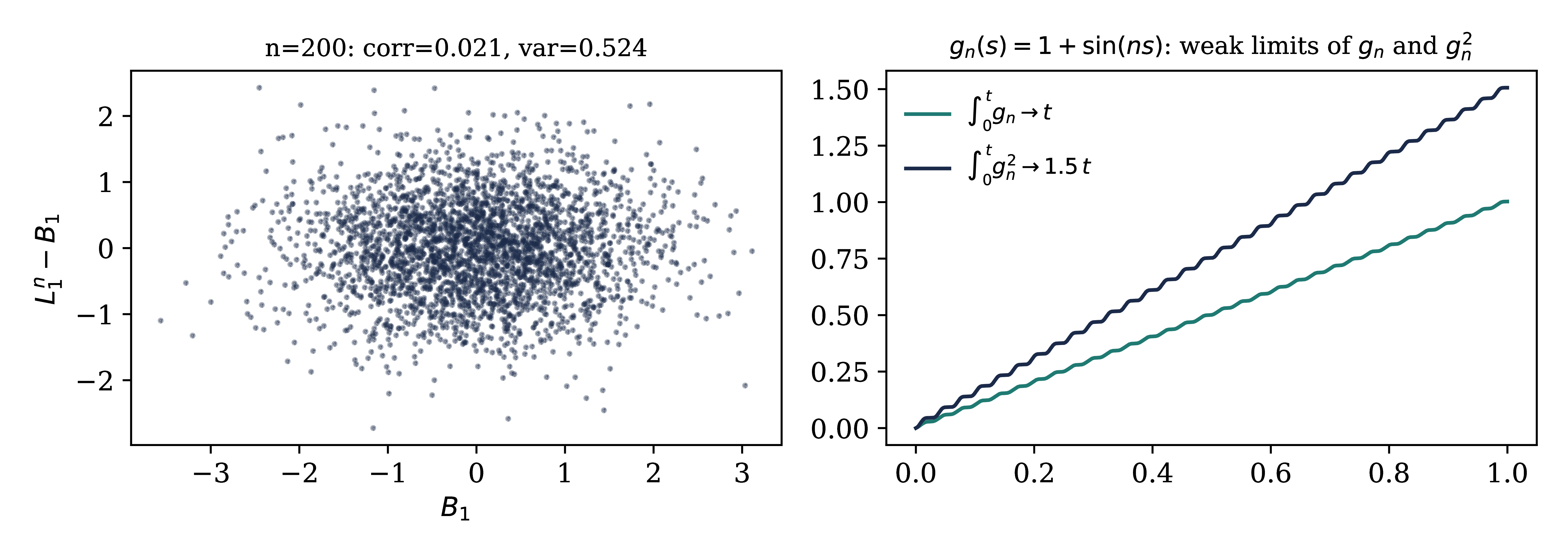
Left: \((B_1, L^n_1 - B_1)\), \(n = 200\): correlation \(\approx 0\), variance of the gap \(\approx \frac{1}{2}\) — the residual does not vanish and is orthogonal to \(B\). Right: \(\int_0^t g_n \to t\) but \(\int_0^t g_n^2 \to \frac{3}{2} t\).

A limit by compactness could carry an extra orthogonal martingale. Here the density excludes it: the filtration is Brownian under the reference.

The renormalised field equation

Theorem. (integration by parts) \(G (\varphi) = g (\langle \varphi, h_1 \rangle, \ldots, \langle \varphi, h_k \rangle)\), \(g \in C_b^{\infty}\), \(h, h_i\) smooth:

\(\displaystyle \lim_N \mathbb{E} \left[ G (\iota_N \Phi^N_{\infty}) \langle \mu_N \Phi^N_{\infty} + \frac{\lambda}{3} (\Phi^N_{\infty})^3, j_N h \rangle \right]\)

\(\displaystyle =\mathbb{E}_{\nu} [D_h G (\Phi) - G (\Phi) \langle \Phi, (q_0 - \Delta) h \rangle] .\)

Proof: Gaussian integration by parts in \(\mathrm{e}^{- V_N - \frac{1}{2} \langle \varphi, K_{q_0} \varphi \rangle}\); tightness and uniform moments.

The terminal case of the DS equations of Lecture 5.
The renormalised cube \(\mu_N \Phi + \frac{\lambda}{3} \Phi^3\) is identified only tested in expectation, not as a random distribution.
Limiting force without terminal representative: not proved.
At every finite resolution the force is explicit: \(F_q = K_q Z_q - \bar{\mathcal{F}}_q (Y_q)\).

The field equation at resolution \(q\)

In the limit: \(\eta_q = K_q \Phi_q - (q - q_0) \psi_q\), \(F_q = K_q (\psi_q - \Phi_q)\), \(J_q = (q - q_0) C_q \to I\).

Theorem. For every \(q\), with no renormalisation constant, pathwise as distributions,

\(\displaystyle K_{q_0} \Phi_q = J_q F_q + \eta_q, \qquad \mathbb{E}D_{J_q h} G (\Phi_q) =\mathbb{E} [G (\Phi_q) \langle \eta_q, h \rangle] .\)

\(\langle F, h \rangle\), \(\langle \eta, h \rangle\) are martingales, and \(\| \langle F_q + \bar{\mathcal{F}}_q (Y_q), h \rangle \|_{L^2} \lesssim \|h\|_{H^2} q^{- 1 / 4}\).

Proof of DS: \(\eta_q =\mathbb{E}_q B_{q - q_0}\) and \(\Phi_q = J_q \Phi_{\infty} + C_q B_{q - q_0}\): Gaussian integration by parts in \(B\).
The renormalised cube is an observable: the unique martingale in the class of the explicit \(- \bar{\mathcal{F}}_q (Y_q)\).
\(q \to \infty\) recovers the integration by parts formula. Not proved: that \(F\) is closed.

Quartic tails: the tilt

Hairer–Steele proved quartic tails by tilting the dynamics. Here: the filter is available for every prior, and the noise bound does not depend on the prior.

Let \(\hat{\nu} \propto \mathrm{e}^{h \langle \varphi, f \rangle} \nu_N\). This is the flow restarted at \((q_0, hC_{q_0} f)\). Shift the coordinate:

\(\displaystyle K_q Y_q + \bar{\mathcal{F}}_q (Y_q) = K_q \Phi_q + hf, \quad Z_q = \hat{\psi}_q - Y_q .\)

The system is the same, \(TZ_T \to 0\) at fixed \(N\), and the field equation gains \(hf\): the noise gains \(d_q = hC_q f\), \(\|d_q \|_{\infty} \leqslant |h| \|f\|_{\infty} / q\).

So UV stability holds on \([q_h, \infty)\) when \(q_h^{3 / 2} \geqslant 70 \lambda^{1 / 2} |h| \|f\|_{\infty}\): where the cube at its threshold, \(qr_q\), dominates the source.

An exact identity, with no cube and no derivative: \(\hat{\Phi} = Y_q + Z_q + (\eta_q - B_{q - q_0}) / (q - q_0)\).

Quartic tails: closing

Test the identity with \(f\), \(\|f\|_{\ast} = \|f\|_1 + \|f\|_2 + \|f\|_{\infty} = 1\), and average over \([q_h, 2 q_h]\), \(X = \langle \hat{\Phi}, f \rangle\):

\(\displaystyle \hat{\mathbb{E}} |X| \leqslant Cr_{q_h} + C \leqslant C (1 + |h|)^{1 / 3} .\)

As \(L (h) = \log \mathbb{E} \mathrm{e}^{h \langle \Phi, f \rangle}\) has \(L' (h) = \hat{\mathbb{E}} X\), we get \(L (h) \leqslant C (|h| + |h|^{4 / 3})\). Chernoff:

\(\displaystyle \mathbb{E} \exp (\beta \langle \Phi, f \rangle^4 /\|f\|_{\ast}^4) \leqslant C, \quad \sup_N \mathbb{E} \exp (\beta_{\rho} \| \iota_N \Phi \|_{H^{- \rho}}^4) < \infty, \quad \rho > \frac{3}{2} .\)

Gaussian tails at the free threshold. A quadratic tilt \(W = \frac{\beta}{2} \| \iota_N \varphi \|_{H^{- s}}^2\), with boundary term \(DW\), gives \(\sup_N \mathbb{E} \exp (\beta_s \| \iota_N \Phi \|_{H^{- s}}^2) < \infty\), \(s > \frac{1}{2}\).

The quartic moment at \(s\) near \(\frac{1}{2}\) would need spatially resolved sources.

Dyson–Schwinger along the scales

DS along the scales. For \(G = g (\langle \Phi_{q_1}, h_1 \rangle, \ldots, \langle \Phi_{q_k}, h_k \rangle)\), \(q_i \leqslant q\):

\(\displaystyle \mathbb{E} \sum_i \partial_i g \langle J_{q_i} h, h_i \rangle =\mathbb{E} [G \langle \eta_q, h \rangle] =\mathbb{E} [G (\langle \Phi_q, K_{q_0} h \rangle + \langle \bar{\mathcal{F}}_q (Y_q), J_q h \rangle)] + O (q^{- 1 / 4}) .\)

So the explicit force \(\bar{\mathcal{F}}_q (Y_q)\) closes the hierarchy at large \(q\), up to an error which vanishes as \(q \to \infty\).

Uniqueness in law and the variational formula

Scalar form. \(A_t = A (t, x_t)\) solves

\(\displaystyle A_t = \int_t^{\infty} \left( e_s (Y_s) + \frac{1}{2} \|Z_s \|_2^2 \right) \hspace{0.17em} \mathrm{d} s + \int_t^{\infty} \langle Z_s, \hspace{0.17em} \mathrm{d} W_s \rangle .\)

With the forward equation \(\hspace{0.17em} \mathrm{d} P = (Y + Z) \hspace{0.17em} \mathrm{d} s + \hspace{0.17em} \mathrm{d} W\) this has uniqueness in law: Girsanov removes \(Z\), pathwise uniqueness gives \(\mathbb{R}\), and the scalar equation gives the density. \(Z\) is the feedback \(m (x) - y (x)\).

Renormalised variational formula. The Gibbs principle over \(\mathbb{R}\):

\(\displaystyle - \log \int \mathrm{e}^{- O} \hspace{0.17em} \mathrm{d} \nu =\mathcal{G} (O) -\mathcal{G} (0), \quad \mathcal{G} (O) = \inf_u \mathbb{E} \left[ O (Y^u_{\infty}) + \int_{q_0}^{\infty} \left( e_s (Y^u_s) + \frac{1}{2} \|u_s \|_2^2 \right) \hspace{0.17em} \mathrm{d} s \right],\)

\(\hspace{0.17em} \mathrm{d} Y^u = (b (Y^u) + H (Y^u) u) \hspace{0.17em} \mathrm{d} s + H (Y^u) \hspace{0.17em} \mathrm{d} W\), \(Y^u_{q_0} = 0\). Minimiser for \(O = 0\): \(u = Z\). No infinite constant, no initial law to optimise.

What is not proved

The vector FBSDE alone: \(Z\) need not be a gradient. It would suffice that any solution has a Lipschitz decoupling field: a pointwise bound on \(\text{Cov}_q (x)\), or high-scale contraction with non-degeneracy. Only \(L^2 (\text{HS})\) control is available.
Strong solutions: is the Polchinski process adapted to \(W\)? The same bound. Allinger–Mitter does not apply, as \(\| \Phi \|_2 = \infty\).
Tails: the quartic moment at \(s\) near \(\frac{1}{2}\).
Axioms: reflection positivity holds on the lattice and passes to \(\nu\) for every coordinate reflection (standard; exercise); rotation invariance and clustering need infinite volume.
Infinite volume: the force and its Burgers flow are intensive, but the entropy and the defect are extensive, so estimates must be made local. The noise from infinity in the nonlocal \(\Xi\) must also be controlled.

Summary of the course

Wightman \(\to\) Euclidean (L1) \(\to\) free field (L2) \(\to\) stochastic quantisation, scale decomposition (L3) \(\to\) Polchinski, FBSDE, variational problem (L4) \(\to\) field equation at every resolution, sub-Gaussian noise (L5) \(\to\) \(\Phi^4_3\) through the FBSDE in forecast coordinates (L6–7).

Lecture 4 (formal)	Lectures 6–7	in the limit
forecast \(\psi_t =\mathbb{E}_t \Phi_T\)	\(\psi = Y + Z\)	closed martingale
response \(H_t = \text{Cov}_t\)	\(\text{Cov} = H (Y) + \Xi\)	conditional covariance
\(\mathcal{F}_t\), force equation	\(\bar{\mathcal{F}}_q\) explicit, defect \(\mathcal{D}\)	deterministic coefficients
force \(F_t\)	\(K_q Z_q - \bar{\mathcal{F}}_q (Y_q)\)	observable at finite \(q\)
DS equation	integration by parts	tested in expectation

UV stability \(=\) an explicit force predicts the conditional mean up to a small error. So the measure is an explicit density over an explicit flow, with that error as the optimal control.