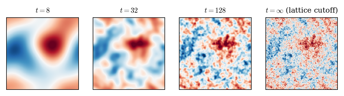
Heat profile on \(\mathbb{T}^2\),
\(m = 4\): \(t = 8, 32, 128\)
and the lattice cutoff, same white noise.
The martingale reveals finer and finer details; the large scales are fixed at low resolution.
A Constructive Introduction to Quantum Field Theory
Stochastic observables, the Polchinski flow, FBSDEs
Massimiliano Gubinelli | University of Oxford
SISSA lectures, Lecture 3 — notes: Lecture 3, §§4–10
So far. A Euclidean field is a measure on \(\mathcal{S}' (\mathcal{M})\); the GFF \(\mu_m\) is its Gaussian part; local operators are functions of \(\varphi\). Wick powers \(: \varphi^n\): are random distributions iff \(n (d - 2) < d\), and not even tight otherwise.
Today. Index everything by a resolution \(t \in [0, \infty)\).
The GFF as the terminal value of a martingale of smooth fields; observables \(=\) martingales.
Interactions: the Polchinski equation and its FBSDE; the force is an observable.
The FBSDE in force coordinates \(\Rightarrow\) the Wetterich equation.
Variational structure: Boué–Dupuis, HJB, infinite volume.
Additional material: products and OPE, flatness, counterterms for \(\Phi^4_3\), DS equations at every scale.
Wilson–Kadanoff: physics is organised scale by scale. The measure-on-\(\mathcal{S}'\) picture hides this, and forces singular objects from the start.
Observe the field at resolution \(t\): a smooth function \(\varphi_t\). Information at resolution \(t\): \(\mathcal{F}_t = \sigma (\varphi_s : s \leq t)\).
A physical quantity is not a random variable but a consistent family of finite-resolution estimates, i.e. a martingale.
Slogan
Observables are martingales in the filtration of finite-resolution measurements. They need not have a terminal value.
Caveat. Statements marked
Setting: covariance profiles and observables
Lecture 3
Definition. A covariance profile is a family \((Q_t)_{t \geq 0}\) of symmetric, translation invariant operators with \(Q_0 = 0\), \(\dot{Q}_t := \partial_t Q_t \geq 0\), \(Q_t \to C = (m^2 - \Delta)^{- 1}\), and smooth kernels for \(t < \infty\).
Heat profile:
\(\dot{Q}_t\) lives on distances \(\lesssim 1 / t\); \(Q_t\) keeps the modes \(|k| \lesssim t\): \(t\) is a momentum scale.
Others: sharp Fourier cutoff \(\mathbb{1}_{|k| \leq t} (|k|^2 + m^2)^{- 1}\); finite range decompositions, \(\dot{Q}_t (x, y) = 0\) for \(|x - y| \geq 1 / t\).
Notation: \(c_t = Q_t (x, x)\), \(Q_{T, t} = Q_T - Q_t\). For \(d \geq 2\), \(c_t \to \infty\) (\(\frac{1}{2 \pi} \log t\) in \(d = 2\), \(\asymp t^{d - 2}\) in \(d \geq 3\)).
\(W\) cylindrical Brownian motion on \(L^2 (\mathcal{M})\),
Proposition. \(X_t\) is a smooth Gaussian field, \(\text{Law} (X_t) = \mu^{Q_t}\); \((X_t (x))_t\) is a continuous martingale with \(\mathrm{d} \langle X (x), X (y) \rangle_t = \dot{Q}_t (x, y) \hspace{0.17em} \mathrm{d} t\); \(X_t \to X_{\infty}\) in \(H^{- s}_{\text{loc}}\), \(s > \frac{d}{2} - 1\), with \(\text{Law} (X_{\infty}) = \mu_m\); \(X_T - X_t \perp \mathcal{F}_t\), with law \(\mu^{Q_{T, t}}\).
The GFF is the terminal value of a Gaussian martingale of smooth fields.
Proof (torus). \(X_t = \sum_n \left( \int_0^t \dot{q}_n (s)^{1 / 2} \mathrm{d} B^n_s \right) e_n\): independent Gaussian martingales, variance \(q_n (t) \uparrow q_n (\infty)\); then as in Lecture 2.
Heat profile on \(\mathbb{T}^2\),
\(m = 4\): \(t = 8, 32, 128\)
and the lattice cutoff, same white noise.
The martingale reveals finer and finer details; the large scales are fixed at low resolution.
\(\mathbb{E}_t =\mathbb{E}[\hspace{0.17em} \cdot \hspace{0.17em} |\mathcal{F}_t]\).
Definition.
\(Y \in L^1 (\mathcal{F}_{\infty})\) gives a closed observable \(O_t =\mathbb{E}_t Y\).
The point: observables need not be closed. \(X_t (x)\), \(d \geq 2\), diverges, yet is a perfectly good family of estimates.
Asymptotic uniqueness
(a) \(\|O^1_t - O^2_t \|_{L^1} \to 0 \Rightarrow O^1 = O^2\).(b) \(N\) adapted, \(\|N_t - O_t \|_{L^1} \to 0 \Rightarrow O_s = \lim_t \mathbb{E}_s N_t\).
Proof. \(\mathbb{E}_s\) is an \(L^1\) contraction.
An observable is determined by its asymptotics.
A germ of \(O\): functionals \(\ring{O}_t\) of smooth fields with \(\|O_t - \ring{O}_t (X_t)\|_{L^1} \to 0\). A germ determines \(O\).
\(O (x)\) is local if it has germs
Germs are not unique: this freedom is the freedom of choosing counterterms.
Example. \(: X^n_t : (x) = H_n (X_t (x) ; c_t)\) is a local observable in every \(d\) (more later), although \(: \varphi^n\): does not exist as a random distribution when \(n (d - 2) \geq d\).
Interactions: the Polchinski equation and FBSDEs
Lecture 3
Finite volume \(\mathbb{T}^d_L\), terminal resolution \(T < \infty\) (UV cutoff), interaction \(V_T\) bounded below, e.g.
Definition.
The interaction felt at resolution \(t\) once the scales \([t, T]\) are integrated out; \(V_0 (0) = - \log Z_T\) is the free energy.
Proposition.
At every resolution the field is again a Gibbs measure: reference \(Q_t\), potential \(V_t\).
The measure-valued martingale \(t \mapsto \mu_t^{X_t}\) goes from \(\nu_T\) (\(t = 0\)) to \(\delta_{X_T}\) (\(t = T\)): a stochastic localisation of \(\nu_T\) (Eldan), adapted to the covariance profile.
Proof of the marginals. Under \(\mathbb{P}_0\), \(X_T = X_t + (X_T - X_t)\) with independent increment \(\sim \mu^{Q_{T, t}}\), so
Theorem.
Proof. \(u_t = \mathrm{e}^{- V_t} = \mathrm{e}^{\frac{1}{2} \Delta_{Q_{T, t}}} u_T\), \(\Delta_Q = \text{Tr} (QD^2)\), solves the backward heat equation \(\partial_t u_t = - \frac{1}{2} \text{Tr} (\dot{Q}_t D^2 u_t)\). Insert \(D^2 u = (DV \otimes DV - D^2 V) u\).
Nonlinear term: generates new, nonlocal interactions: trees. |
Trace term: contracts pairs of fields with the shell covariance \(\dot{Q}_t \hspace{0.17em} \mathrm{d} t\): loops. |
A backward Hamilton–Jacobi equation; \(u = \mathrm{e}^{- V}\) is a Cole–Hopf transform.
Theorem.
The effective force \(F\) is a \(\mathbb{P}\)-martingale: an observable field of the interacting theory.
Proof. Density process \(M_t = Z_T^{- 1} \mathrm{e}^{- V_t (X_t)}\). Itô \(+\) Polchinski: no drift, \(\mathrm{d} M_t = - M_t \langle DV_t (X_t), \dot{Q}_t^{1 / 2} \mathrm{d} W_t \rangle\). Girsanov: \(W^{\mathbb{P}}_t = W_t + \int_0^t \dot{Q}_s^{1 / 2} DV_s (X_s) \hspace{0.17em} \mathrm{d} s\). Finally \(DV_t (\phi) = \mu_t^{\phi} (DV_T)\).
Read as an equation for an unknown pair \((\Phi, F)\):
The field is driven forward by a force determined backward from the terminal field.
No Polchinski equation needed; \(\nu_T = \text{Law} (\Phi_T)\) from the solution.
Strategy: solve with renormalised \(V_T\), estimates uniform in \(T\) and volume, take limits.
\(\Phi\) is not an observable (a semimartingale); observables are built from the noise and from \(F\).
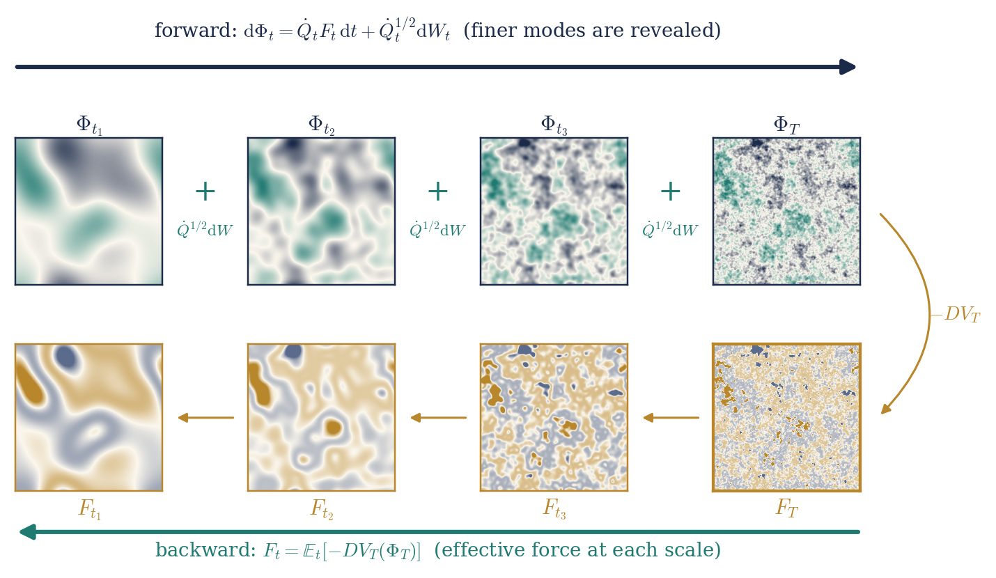
\(\mathbb{T}^2\),
heat profile, same noise. The force is shown to first order in \(\lambda\): \(F_t = - 4 \lambda H_3
(\Phi_t ; c_t)\), each panel in its own units.
At finite \(T\) the force is a closed observable, \(F_t =\mathbb{E}_t [F_T]\), and for \(\Phi^4\) it is local:
As \(T \to \infty\)
\(F\) should converge as an observable. In \(d = 2\) it is closed, \(F_{\infty} = - 4 \lambda : \Phi_{\infty}^3\):. In \(d = 3\) a closed limit \(F_t =\mathbb{E}_t F_{\infty}\) would let the DS identity pass to \(t \to \infty\), and conditioning on \(\sigma (\Phi_{\infty})\) would give an integrable logarithmic derivative of \(\Phi^4_3\) as a function of the field: not expected (Albeverio–Liang–Zegarlinski 2006: the regularised ones do not converge in \(L^2\)). Locality of the limiting force is the crux of the construction.
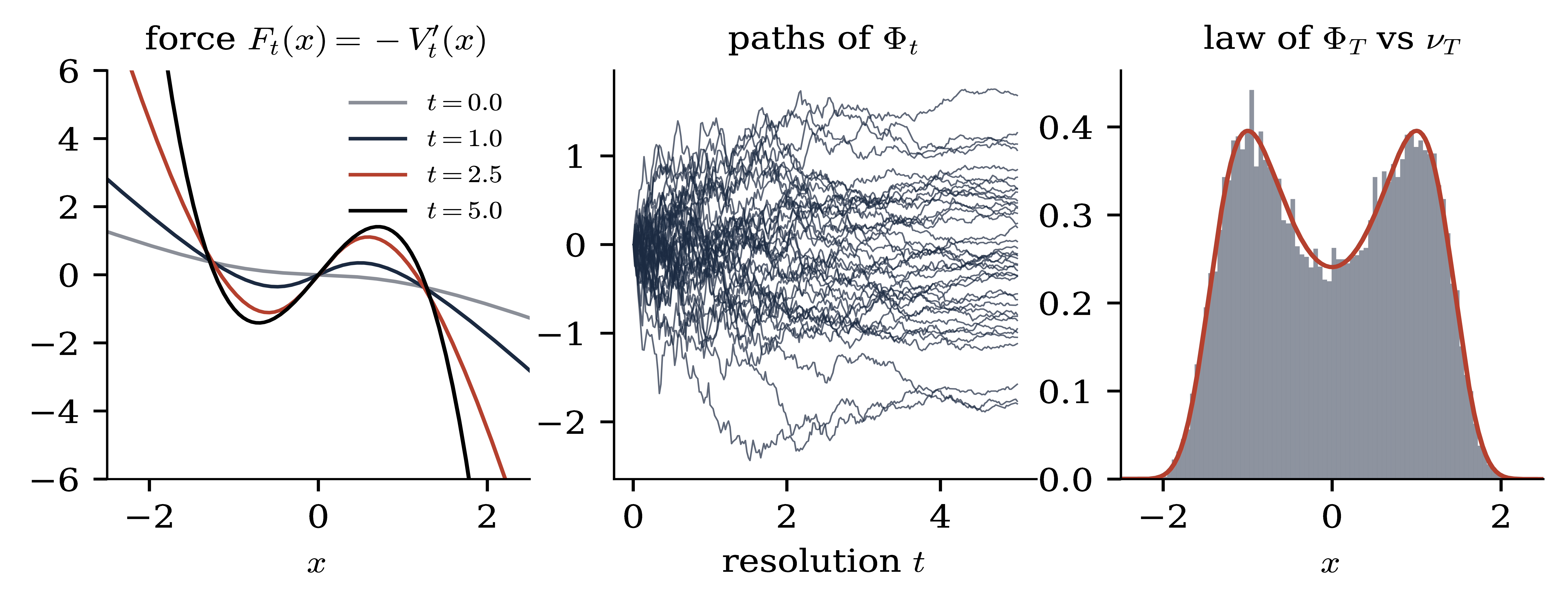
\(Q_t = 1 - \mathrm{e}^{-
t}\), \(T = 5\), \(V_T (x) =
\frac{1}{2} x^4 - \frac{3}{2} x^2\). Left: \(F_t =
- V_t'\), almost linear at low resolution, double well as \(t \to T\). Centre: FBSDE paths split between the wells
(stochastic localisation). Right: histogram of \(\Phi_T\)
vs. the density of \(\nu_T\).
For \(G\) a functional of the terminal field, \(O_t =\mathbb{E}^{\mathbb{P}}_t [G (\Phi_T)] = G_t (\Phi_t)\), \(G_t (\phi) = \mu_t^{\phi} (G)\), and
the backward Kolmogorov equation, a Doob transform of the Gaussian heat equation. Any solution gives an observable, closed at finite \(T\), not necessarily as \(T \to \infty\). The force is \(G = - DV_T\).
Tangent observables. \(V_T^{\theta}\) depending on a coupling, \(U_t = \partial_{\theta} V_t^{\theta}\):
E.g. the running \(: \varphi^4\): for \(\theta = \lambda\): observables conjugate to the coordinates of theory space.
Differentiating Polchinski, \(F_t = - DV_t\) solves the backward viscous Burgers equation
Cole–Hopf \(F = D \log u\) linearises it (\(u = \mathrm{e}^{- V}\) solves a heat equation).
Uses only the force: intensive, while \(V_t\) is extensive (\(\sim\) volume). Matters in infinite volume.
Flows for different covariances commute when \(DF\) is symmetric, i.e. \(F\) a gradient. Non-gradient forces (general Wilson–Itô diffusions): curvature.
The FBSDE in force coordinates: the Wetterich equation
Lecture 3
\(S_t := Q_T - Q_t\): the covariance still unresolved; \(\dot{S}_t = - \dot{Q}_t\), \(S_T = 0\). \(\mathrm{d} F_t = \Upsilon_t \hspace{0.17em} \mathrm{d} W_t\).
Pontryagin. Control problem \(\mathrm{d} X = \dot{Q}_t^{1 / 2} (u \hspace{0.17em} \mathrm{d} t + \mathrm{d} W)\), cost \(V_T (X_T) + \frac{1}{2} \int \|u\|^2\). Hamiltonian \(\langle p, \dot{Q}_t^{1 / 2} u \rangle - \frac{1}{2} \|u\|^2\) is state independent \(\Rightarrow\) \(\mathrm{d} p_t = \Upsilon_t \hspace{0.17em} \mathrm{d} W_t\), \(p_T = - DV_T (X_T)\), \(u_t = \dot{Q}_t^{1 / 2} p_t\).
The field \(\Phi\) is the state; the force \(F\) is the costate.
\(F_t (\cdot)\) is the decoupling field, Burgers its quasilinear PDE.
Transport term \(- DF [\dot{Q} F]\) \(\leftarrow\) drift of the state: trees.
Itô term \(- \frac{1}{2} \text{Tr} (\dot{Q}
D^2 F)\) \(\leftarrow\) noise: loops.
Noiseless flow from \(t\) to \(T\): the linear shear \(\Sigma_t : (x, p) \mapsto (x + S_t p, \hspace{0.17em} p)\), the characteristics of the transport part.
Proposition.
a martingale with \(\mathrm{d} \psi_t = \dot{Q}_t^{1 / 2} \mathrm{d} W_t + S_t \hspace{0.17em} \mathrm{d} F_t = (\mathbb{1} + S_t DF_t (\Phi_t)) \dot{Q}_t^{1 / 2} \mathrm{d} W_t\).
Proof. \(F\) martingale \(\Rightarrow \mathbb{E}_t \int_t^T \dot{Q}_s F_s \hspace{0.17em} \mathrm{d} s = S_t F_t\). In the differential, \(\dot{Q}_t F_t \hspace{0.17em} \mathrm{d} t\) cancels with \(\dot{S}_t F_t \hspace{0.17em} \mathrm{d} t\).
\(\Phi_t = \psi_t - S_t F_t\): a martingale (the field observable) minus the drift still expected on the unresolved scales.
Noise of \(\psi\): fresh shell fluctuation \(+\) revision of the forecast. The forward–backward coupling moves from the drift to the volatility.
\(\psi\) is the interaction picture w.r.t. the classical dynamics.
Invert \(x \mapsto \psi = x + S_t F_t (x)\): \(x = \psi + S_t \mathscr{F}_t (\psi)\), \(\mathscr{F}_t (\psi) := - F_t (x)\). Response and regulator:
Theorem.
\(\psi_T = \Phi_T\). No drift; covariance \(\mathcal{C}_t = H_t \dot{\mathscr{R}}_t H_t^{\ast}\). The decoupling field solves the pure diffusion equation
Proof. \(\mathbb{1} + S_t DF_t = H_t S_t^{- 1}\); \(\mathscr{F}_t (\psi_t)\) is a martingale and \(\psi\) has no drift: Itô.
Compare with Burgers:
The transport term is absorbed exactly: dropping the Itô term, \(\mathscr{F}_t = DV_T\) does not move. All trees live in the coordinate change \(x = \psi + S_t \mathscr{F}_t (\psi)\).
Loops come only from the quadratic variation \(\mathcal{C}_t\) of the forecast; the nonlinearity has moved into its field dependence.
No gradient structure, no Gaussian convolution used: valid for any FBSDE with a Markov martingale force, whenever the coordinate change is invertible.
Proposition.
So \(H_t > 0\), \(\mathbb{1} + S_t DF_t\) is always invertible, and \(H_t \leq S_t\) for convex \(V_T\) (Brascamp–Lieb).
The forecast coordinates are the first two conditional moments of the stochastic localisation: \((\psi_t, \text{Cov}_t) = (\mathbb{E}_t \Phi_T, \text{Cov}_t \Phi_T)\). Since \(\mathbb{E}_t [\Phi_T \otimes \Phi_T] = \psi_t \otimes \psi_t + \text{Cov}_t\) is a martingale,
Gaussian reference: \(S_t \dot{\mathscr{R}}_t S_t = \dot{Q}_t\).
Two-component field, \(V_T\)
a tilted double well (contours: \(\nu_T\)). Path \(\Phi_t\), forecast
\(\psi_t = \Phi_t + S_t F_t\), conditional
law \(\mu_t^{\Phi_t}\) and \(2
\sigma\) ellipse of \(\text{Cov}_t\);
open circle: \(\Phi_T\). The conditional law
localises on one well.
\(F_t = - DV_t\): the graph \(\{(x, - DV_t (x))\}\) is a Lagrangian submanifold of (field, force) space. The shear \(\Sigma_t\) is symplectic (\(S_t\) symmetric), and the image is a graph over \(\psi\) (\(x \mapsto x + S_t F_t (x)\) is \(S_t \hspace{0.17em} D\) of a strictly convex function). Hence
Generating function: the Moreau transform
optimality: \(x = \psi + S_t D \Gamma_t (\psi)\), \(DV_t (x) = D \Gamma_t (\psi)\). Well defined: \(\frac{1}{2} \langle x, S_t^{- 1} x \rangle - V_t (x)\) has Hessian \(S_t^{- 1} \text{Cov}_t S_t^{- 1} > 0\).
Left: \(\Sigma_t\)
maps the graph of \(F_t = - V_t'\) to the graph of
\(- \Gamma_t'\) over the forecast. Right: \(V_T\), \(V_t\) and \(\Gamma_t\)
(\(t = 1.2\), \(T = 5\)).
Theorem.
Equivalently, for the effective average action \(\Gamma^{\text{EAA}}_t = \Gamma_t + \frac{1}{2} \langle \psi, Q_T^{- 1} \psi \rangle\),
from the bare action (\(t = T\), \(\mathscr{R}_T = \infty\)) to the 1PI effective action of \(\nu_T\) (\(t = 0\), \(\mathscr{R}_0 = 0\)).
Proof. \(D_v \text{Tr} (\dot{\mathscr{R}} H) = - \text{Tr} (\mathcal{C} \hspace{0.17em} D^2 \mathscr{F}) [v]\) by symmetry of \(D^3 \Gamma\), so the force equation reads \(D \left( \partial_t \Gamma - \frac{1}{2} \text{Tr} (\dot{\mathscr{R}} H) \right) = 0\). The constant: envelope theorem \(+\) Polchinski.
Every object in the Wetterich equation is an observable of the Polchinski process.
| Wetterich | FBSDE |
| field argument \(\psi\) | forecast \(\psi_t =\mathbb{E}_t [\Phi_T]\) |
| \(D \Gamma_t (\psi_t)\) | minus the costate, \(\mathbb{E}_t [DV_T (\Phi_T)]\) |
| propagator \((D^2 \Gamma^{\text{EAA}}_t + \mathscr{R}_t)^{- 1}\) | conditional covariance \(\text{Cov}_t\) |
| regulator \(\mathscr{R}_t = S_t^{- 1} - Q_T^{- 1}\) | precision of the unresolved shell minus the prior's |
| \(\partial_t \Gamma_t\) | \(\frac{1}{2} \text{Tr} [\dot{\mathscr{R}}_t (\text{Cov}_t - S_t)]\) |
Driven by interacting minus free conditional covariance; one-loop exact, with the full propagator; in the Gaussian case only the constant flows. Wetterich 1993; Morris 1994; Berges–Tetradis–Wetterich 2002
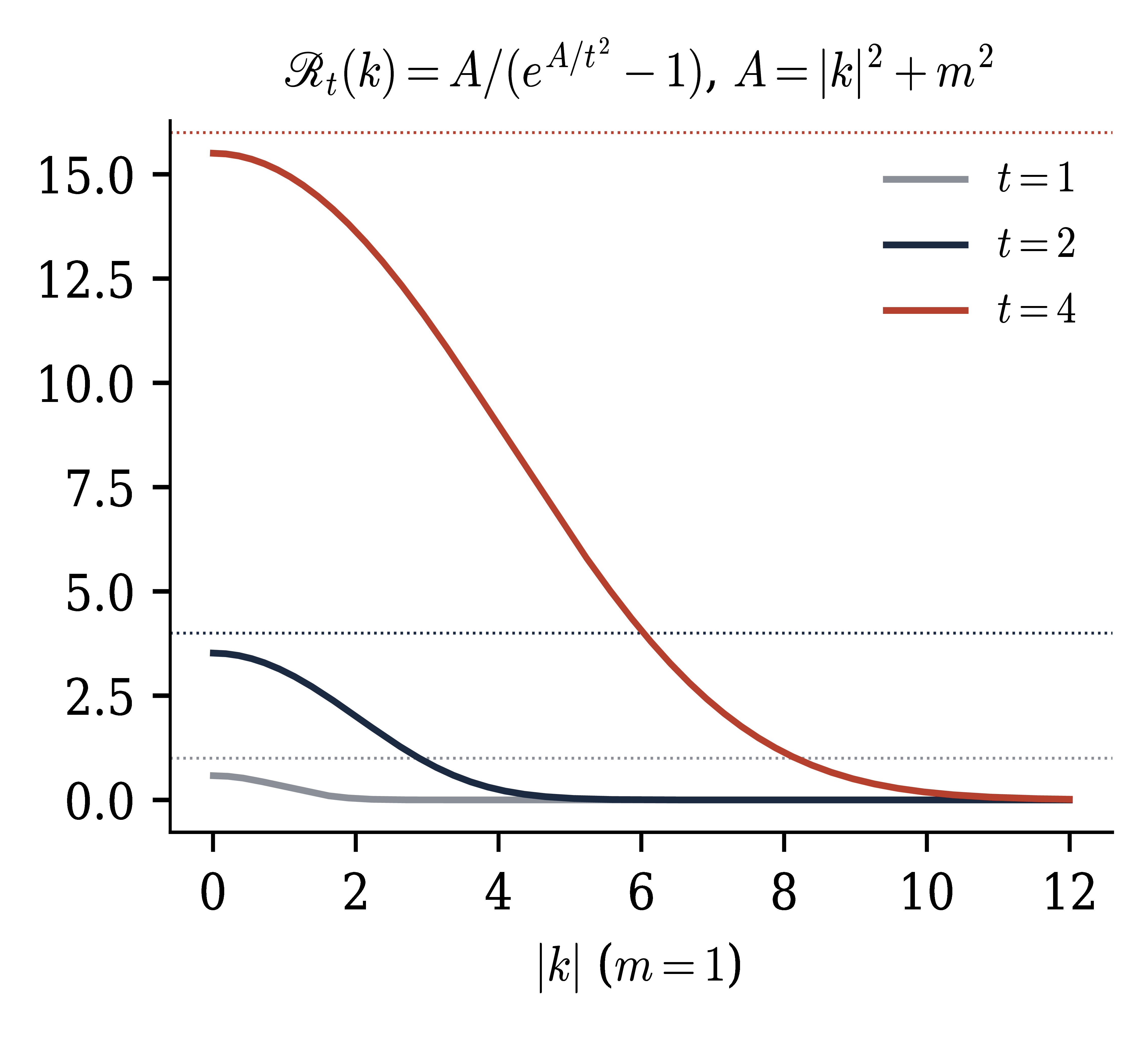
For \(T = \infty\), \(S_t = C (1 - \mathrm{e}^{- A / t^2})\) and
The exponential regulator of the functional RG. Other profiles give other regulators, e.g. the mass regulator \(\mathscr{R}_t = t^2\). |
|
Constrained free energy. Gibbs variational principle for the conditional law:
the free energy of the unresolved shell, constrained to the forecast. \(V_t\) is the value function; \(\Gamma_t\) is its Moreau transform.
Tree level. Drop the Itô term: \(\Gamma_t = V_T\), and the Moreau transform becomes the Hopf–Lax formula
which solves \(\partial_t V = \frac{1}{2} \langle DV, \dot{Q} DV \rangle\): the saddle point of the Gaussian convolution. The minimiser solves the classical field equation \(S_t^{- 1} (y - x) + DV_T (y) = 0\) in the shell \([t, T]\); expanding in \(V_T\) gives exactly the tree diagrams.
Variational structure
Lecture 3
\(\mathbb{H}_a\): adapted drifts with \(\mathbb{E} \int_0^T \|u_s \|^2 < \infty\); \(X^u = X + \int_0^{\cdot} \dot{Q}_s^{1 / 2} u_s \hspace{0.17em} \mathrm{d} s\).
Theorem.
Optimal feedback \(u^{\ast}_s = - \dot{Q}_s^{1 / 2} DV_s (X^{u^{\ast}}_s)\), \(\text{Law} (X^{u^{\ast}}_T) = \nu_T\). \(V_t\) is the value function; Polchinski is the HJB equation.
Proof (verification). Itô \(+\) Polchinski:
Euler–Lagrange. Perturb \(u \to u + \varepsilon v\):
Entropy. \(\frac{1}{2} \mathbb{E}_0 \int \|u\|^2 \geq \text{Ent} (\text{Law} (X^u) | \text{Law} (X))\): a pathwise lift of the Gibbs principle \(- \log Z_T = \inf_{\nu} \{ \int V_T \hspace{0.17em} \mathrm{d} \nu + \text{Ent} (\nu | \mu^{Q_T})\}\). Useful because adapted drifts can be built scale by scale, as functionals of \(X\).
Generating functional:
Bounds uniform in \(T\) \(\Rightarrow\) tightness, moments, identification of limits.
\(\Phi^4_3\). The leading drift \(u_s \approx - 4 \lambda \dot{Q}_s^{1 / 2} : X_s^3\): has divergent cost,
Change variables \(u = - 4 \lambda \dot{Q}^{1 / 2} : X^3 : + r\), then paracontrolled changes of variables: the singular terms become explicit polynomials in Wick powers of \(X\), cancelled by the counterterms, and the remainder is coercive. Uniform control in Besov/paracontrolled norms \(=\) construction of \(\Phi^4_3\). Barashkov–Gubinelli, Duke 2020; EJP 2021
On \(\mathbb{T}^d_L\), \(V_0 (0)\) and \(V_t\) are extensive (\(\sim L^d\)). Three intensive objects survive:
the force. For \(V_T = \int v_T (\varphi)\), on \(\mathbb{R}^d\):
Everything is local; infinite-volume limits should solve this. Uniqueness of solutions \(\leftrightarrow\) uniqueness of the theory; non-uniqueness expected at phase transitions (\(\Phi^4_2\), deep double well).
the Burgers flow of the force;
differences of free energies \(\mathcal{W}_T^{(L)} (f)\), \(f\) local: bounded as \(L \to \infty\); basis of the infinite-volume analysis of \(\Phi^4_2\) and \(\exp (\Phi)_2\).
Estimates must be local (weighted norms, volume-independent constants): the analogue of “coming down from infinity”. Barashkov–Gubinelli, PMP 2023; Glimm–Jaffe–Spencer 1975
Additional material
Lecture 3
Recall \(\partial_c H_n (a ; c) = - \frac{1}{2} \partial_a^2 H_n\), \(\partial_a H_n = nH_{n - 1}\).
Proposition. For every \(d\), \(n\), \(x\): \(: X^n_t : (x) := H_n (X_t (x) ; c_t)\) is a continuous martingale, \(\mathrm{d} \hspace{0.17em} : X^n_t : (x) = n \hspace{0.17em} : X^{n - 1}_t : (x) \hspace{0.17em} \mathrm{d} X_t (x)\), and
Proof. Itô: the drift is \((\frac{1}{2} \partial_a^2 + \partial_c) H_n \hspace{0.17em} \dot{c}_t = 0\).
Lecture 2: \(: \varphi^n\): exists iff \(n (d - 2) < d\). As observables, Wick powers exist in every \(d\), unsmeared.
For \(n (d - 2) \geq d\), \(0 \leq f \mathrel{\not\equiv} 0\), \(: X^n_t : (f)\) is unbounded in \(L^2\) and (Paley–Zygmund) not tight: no terminal value; the observable is the whole family.
The singularity has moved to products at coincident points.
Definition. \(O^1 \star O^2\) is the observable with \(\|(O^1 \star O^2)_t - O^1_t O^2_t \|_{L^1} \to 0\); unique, and \((O^1 \star O^2)_s = \lim_t \mathbb{E}_s [O^1_t O^2_t]\).
Proposition. If \(O^1, O^2\) are continuous, square integrable on bounded intervals, and \(\mathbb{E} \int_0^{\infty} | \mathrm{d} \langle O^1, O^2 \rangle_s | < \infty\), then
Proof. \(O^1 O^2 - \langle O^1, O^2 \rangle\) and \(\mathbb{E}_t \langle O^1, O^2 \rangle_{\infty}\) are martingales.
\(\langle \textbf{X} (x), \textbf{X} (y) \rangle_t = Q_t (x - y)\) is deterministic. Heat profile, \(d \geq 2\): the condition holds iff \(x \neq y\), and then
The correct two-point function, without ever discussing the regularity of \(X_{\infty}\). For \(x = y\): no product, since \(c_t \to \infty\).
OPE. At every fixed resolution, as \(y \to x\),
i.e. \(\textbf{X} (x) \star \textbf{X} (y) = G (x - y) \mathbb{1} + : \textbf{X}^2 : (x) + o (1)\): the Wick square is the regular part of the product.
For \(x \neq y\),
Wick's theorem at the level of observables.
The coefficients \(G (x - y)^j\) carry all singularities; the observables on the right have regular limits as \(y \to x\).
\(O^1, O^2\) with germs supported in \(U^1_{1 / t}\), \(U^2_{1 / t}\), \(\text{dist} (U^1, U^2) > 0\): the covariation \(\langle DO^1_t, \dot{Q}_t \hspace{0.17em} DO^2_t \rangle \mathrm{d} t\) sees \(\dot{Q}_t\) only between the supports.
Finite range decomposition: it vanishes for large \(t\), so the product exists and is asymptotically the pointwise product. Heat profile: exponentially small.
Observables on disjoint regions multiply freely; products at the same point need renormalisation.
Factorisation algebra
This is the structure of a factorisation algebra of observables (precise axioms not established here).
Bauerschmidt–Brydges–Slade, LNM 2242 (finite range decompositions)
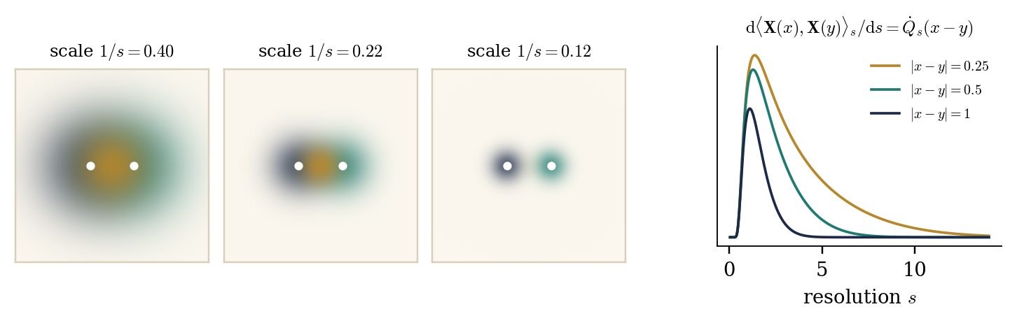
Left: kernels of \(\dot{Q}_s^{1 / 2}\) at \(x\) and
\(y\); their overlap integrates to \(\dot{Q}_s
(x - y) = \mathrm{d} \langle \textbf{X} (x), \textbf{X} (y)
\rangle_s
/ \mathrm{d} s\). Right: negligible for \(s \gg 1
/ |x - y|\); total \(G (x - y)\). As \(y \to x\) the mass escapes to \(s \to
\infty\).
\(\mathcal{R}_S (V) = - \log (\mu^S \ast \mathrm{e}^{- V})\). Since \(\mu^S \ast \mu^{S'} = \mu^{S + S'}\),
an orbit of an abelian semigroup indexed by the cone of positive covariances, nonlinear on \(V\), linear on \(\mathrm{e}^{- V}\). Generators:
Proposition.
Different profiles with the same endpoints are different coordinate systems on the same RG trajectory: they change \(\Phi\) and intermediate observables, not the terminal theory. No holonomy.
Gaussian convolution lowers the Wick ordering: \(V_t = \int [\lambda : \phi^4 :_t + \gamma_T : \phi^2 :_t] + O (\lambda^2)\), the dual of \(\int H_4 (X_t ; c_t)\) being an observable. At second order, \(S = Q_{T, t}\):
\(T \to \infty\) at fixed \(t\), \(d = 3\), \(G (z) \sim (4 \pi |z|)^{- 1}\):
\(k = 1, 2\): finite, nonlocal.
\(k = 3\) (sunset): \(S^3 \sim |z|^{- 3}\); local divergence \(- 48 \lambda^2 (\int S^3) \int : \phi^2 :_t\) (+ const), cancelled by \(\gamma_T = 48 \lambda^2 \int Q_T^3 = \frac{3 \lambda^2}{\pi^2} \log T + O (1)\).
\(k = 4\): vacuum energy \(\sim T\); cancels in \(\nu_T\).
Renormalisation \(=\) choosing \(V_T\) so that \(V_t\) at fixed resolution converges. \(\nu_t \ll \mu^{Q_t}\) expected for \(t < \infty\); the terminal \(\Phi^4_3\) is singular w.r.t. the GFF.
Operators functions of \(A\); \(K = Q_T^{- 1}\), \(J_t = KQ_t\) (heat profile: a heat semigroup, \(\to \mathrm{e}^{- A / t^2}\)).
Theorem.
At \(t = T\): the DS equation \(\mathbb{E}^{\nu_T} [D_h G] =\mathbb{E}^{\nu_T} [G \langle h, K \varphi + DV_T \rangle]\).
Proof. \(\dot{J}_t = K \dot{Q}_t\): drifts cancel. IBP for \(\mu^{Q_t}\) in direction \(J_t h\), using \(\Phi_t \sim \nu_t\).
As \(T \to \infty\), \(K \to A\), and \(\eta_t = K \Phi_t - J_t F_t\) becomes
the Euclidean field equation \(A \varphi = - V' (\varphi) +\)noise, seen at resolution \(t\). No products of distributions: the nonlinearity enters only through the force observable, smeared at scale \(1 / t\). For \(\Phi^4_3\), with \(F_t\) in the role of the renormalised cube, \(t \to \infty\) corresponds to the renormalised DS equation (Gubinelli–Hofmanová 2021).
Compare: stochastic quantisation (Lecture 2)
There the field equation is imposed in an auxiliary time; here it holds at each resolution, and the auxiliary parameter is the resolution itself.
Conditioning an SPDE solution on a scale filtration gives identities of the same shape but with a different noise: the martingale \(J_t \hspace{0.17em} \mathrm{d} F_t\) in \(\mathrm{d} \eta_t\) is essential.
The GFF is the terminal value of a martingale \(X_t\) of smooth fields; observables are martingales, possibly without terminal value.
Interactions: effective potentials \(V_t\) solve Polchinski; the interacting field solves an FBSDE whose force is an observable.
In the forecast coordinate \(\psi_t =\mathbb{E}_t \Phi_T\) the FBSDE has no drift, trees are integrated exactly, and the force flow is pure diffusion; in the gradient case it is Wetterich's equation.
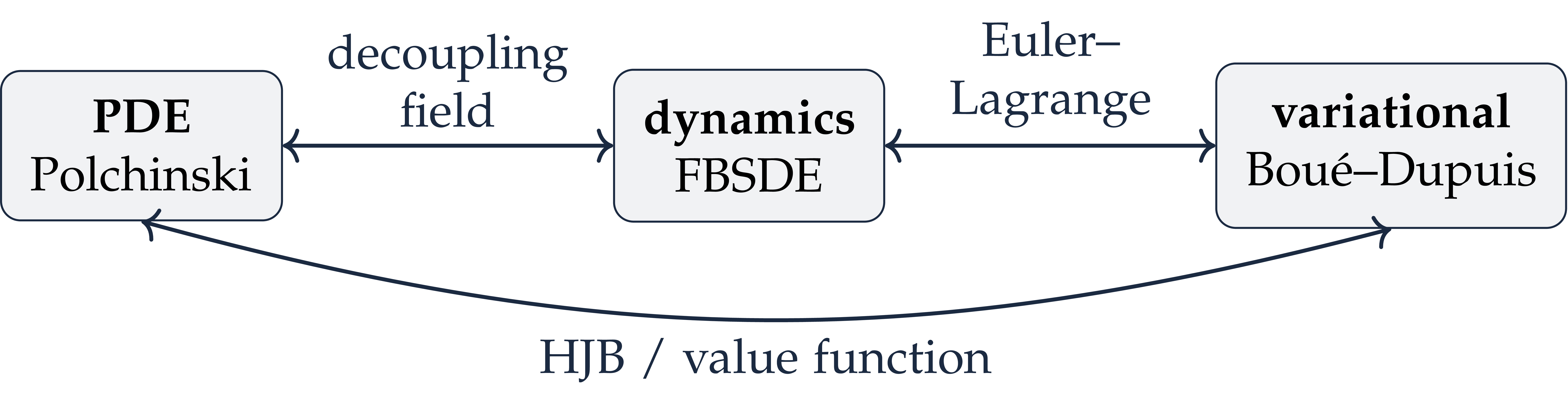
PDE (Polchinski) \(\leftrightarrow\) dynamics (FBSDE) \(\leftrightarrow\) variational principle (Boué–Dupuis).
Products, OPE, counterterms and DS equations all live at finite resolution.
Next
Later lectures (not yet settled): probably a construction of \(\Phi^4_3\) on the torus via the FBSDE.
Exercises (numbering of the notes)
|
Reading
|