Constructive quantum field theory — Lecture 4 (slides)

Lecture 3. Interacting field at resolution \(t\) = solution of the FBSDE

In the forecast coordinate \(\psi_t =\mathbb{E}_t \Phi_T\) the forward equation has no drift and the trees are integrated exactly; the backward half is the Wetterich equation.

Lectures 4–6. Construct \(\Phi^4_3\) on \(\mathbb{T}^3\) with this FBSDE:

1. deterministic renormalisation: an explicit approximate effective action \(\bar{\Gamma}_q\) and its defect (today);

2. a priori estimates for the exact FBSDE in the coordinates of \(\bar{\Gamma}_q\), uniform in the lattice (Lecture 5);

3. removing the cutoffs and identifying the limit (Lecture 6).

G., course notes on \(\Phi^4_3\) via FBSDEs (2026); Bailleul–Chevyrev–G. (in prep.)

• Large mass \(m^2 = q_0\) compared with the coupling: \(\gamma q_0^{- 1 / 2} \ll 1\), \(\gamma = 3 \lambda\). A weak dimensionless coupling on a fixed torus.

• Tightness of the lattice measures in \(H^{- s}\), \(s > \frac{1}{2}\).

• A subsequential limit: an FBSDE on \([q_0, \infty)\), driven by a Brownian motion obtained as the limit of the lattice innovations, whose terminal value has the limiting law.

• A renormalised integration by parts formula.

Not proved: uniqueness, OS axioms, infinite volume.

Other constructions: Glimm–Jaffe 1973; Feldman–Osterwalder 1976; Brydges–Fröhlich–Sokal 1983; Barashkov–G. 2020; G.–Hofmanová 2021

The problem and the exact FBSDE

Lecture 4

\(\Lambda_N = (N^{- 1} \mathbb{Z}/\mathbb{Z})^3\), \(\int f = N^{- 3} \sum_x f (x)\), \(\Delta = \Delta_N\) nearest neighbour. Resolution parameter \(q = q_0 + t^2 \in [q_0, \infty)\):

In Lecture 3 notation (\(T = \infty\), and \(\dot{Q} = \partial_q Q_q\)):

The bubble \(a_2 (q)\) is the coincident-point variance of the shell at resolution \(q\).

\(\gamma = 3 \lambda\), so \(D^2 U (y) = \gamma y^2\) (not the counterterm \(\gamma_T\) of Lecture 3). The Wick ordering is now part of \(\mu_N\).

Theorem. (informal) For \(q_0\) large: explicit \(\mu_N = - 3 \lambda \text{Tr} C + O (\log N)\) such that (a) \(\nu_N\) is tight in \(H^{- s}\), \(s > \frac{1}{2}\); (b) along a subsequence, the forecasts converge to a solution of a limiting FBSDE; (c) the limit satisfies a renormalised integration by parts formula.

The bounds behind (a), (b) are bounds on the error \(Z\) of an approximate forecast, uniform in \(N\): UV stability.

Fixed \(N\). Hidden field \(\Phi_{\infty} \sim \nu_N\), independent Brownian motion \(B\), observations

Proposition. With \(\mathcal{K}_q (p) = \log \int \mathrm{e}^{\langle p, \varphi \rangle - \frac{q - q_0}{2} \| \varphi \|^2} \nu_N (\mathrm{d} \varphi)\):

Proof: Bayes with likelihood \(\exp \{\langle P_q, \varphi \rangle - \frac{q - q_0}{2} \| \varphi \|^2 \}\); Lévy's characterisation; Itô on \(D\mathcal{K}_q (P_q)\).

Proposition. \(\Phi_q := C_q P_q\) and \(F_q := K_q (\psi_q - \Phi_q)\) satisfy

i.e. the FBSDE of Lecture 3 for the mass profile. \(\text{Cov}_q\) is the response \(H^{\text{ex}}_q (\psi_q)\).

• Drift: \(\mathrm{d} (C_q P_q) = - C_q^2 P_q \mathrm{d} q + C_q (\psi_q \mathrm{d} q + \mathrm{d} W_q)\).

• Force: posterior integration by parts, \(p = K_q D\mathcal{K}_q (p) +\mathbb{E}_{\text{post}} [DV_N]\) (posterior with source \(p\)), at \(p = K_q \Phi_q\).

• Same law as Lecture 3: both are the Gaussian law tilted by \(\mathrm{e}^{- V_N} /\mathcal{Z}_N\) of the terminal field; \(\sigma (P) = \sigma (\Phi)\).

At fixed \(N\) the FBSDE is a theorem, and \(W\) is an innovation.

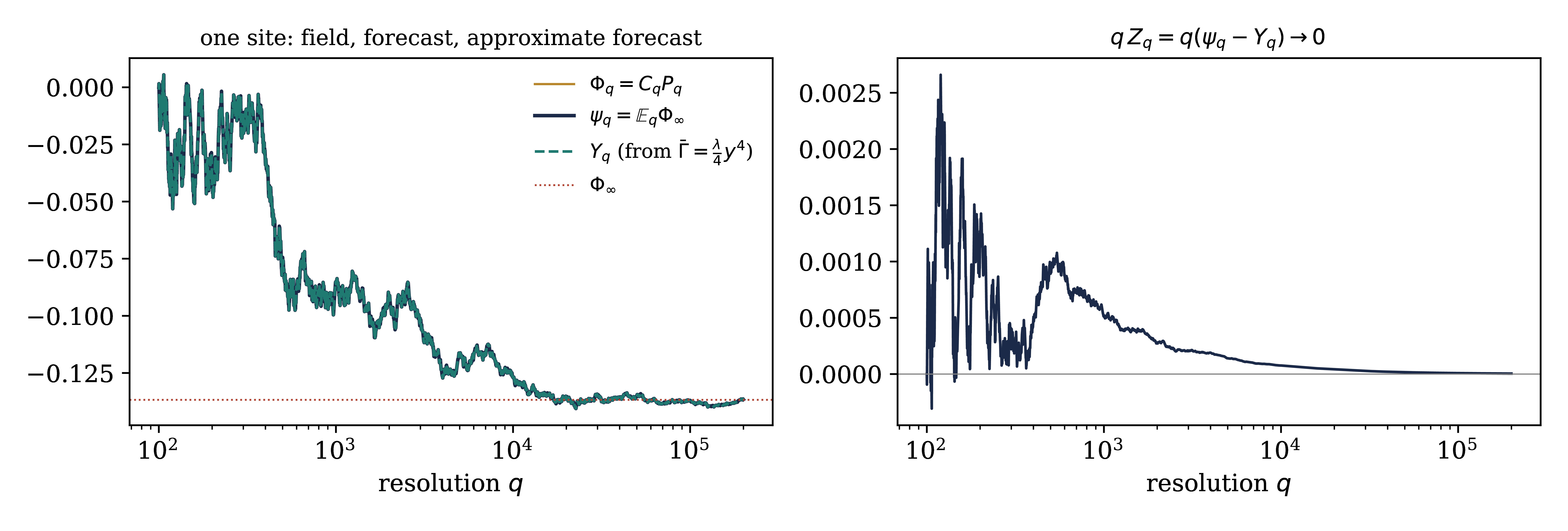
Illustration: \(\nu \propto \mathrm{e}^{- \lambda \varphi^4 / 4} \mu^{1 / q_0}\) on one site, \(\lambda = 2\), \(q_0 = 100\) (\(g_{q_0} = 0.6\)). \(\Phi_q = P_q / q\), the posterior mean \(\psi_q\), and the approximate forecast \(Y_q\) from \(\bar{\Gamma} = \frac{\lambda}{4} y^4\). All converge to the hidden \(\Phi_{\infty}\), and \(qZ_q \to 0\).

The lattice is the only UV cutoff: terminal resolution \(q = \infty\), and \(\Phi_q \to \Phi_{\infty}\).

\(\Psi_q =\mathcal{K}_q^{\ast}\), \(\Gamma_q (y) = \Psi_q (y) - \frac{1}{2} \langle y, K_q y \rangle\), \(H^{\text{ex}}_q (y) = (K_q + D^2 \Gamma_q (y))^{- 1}\).

• Up to a function of \(q\), \(\Gamma_q\) is the \(\Gamma_t\) of Lecture 3; \(\Gamma_q + \frac{1}{2} \langle y, K_{q_0} y \rangle\) is the effective average action with regulator \(\mathcal{R}_q = q - q_0\).

• Coordinates: \(\Phi_q = \psi_q + C_q D \Gamma_q (\psi_q)\) (Lecture 3, \(x = \psi + S \mathscr{F} (\psi)\)).

Proposition. (Wetterich with a mass regulator)

An identity about the unknown \(\nu_N\), not a construction. Strategy: an approximate \(\bar{\Gamma}\) gives approximate forecast coordinates; the error should be driven by the failure of \(\bar{\Gamma}\) to solve Wetterich.

\(\bar{\Gamma}_q\) even, \(\bar{\Psi}_q = \frac{1}{2} \langle y, K_q y \rangle + \bar{\Gamma}_q\) uniformly convex, \(\bar{\mathcal{K}}_q = \bar{\Psi}_q^{\ast}\).

Theorem. (exact, at fixed \(N\))

Proof: \(\partial_q \bar{\mathcal{K}} + \frac{1}{2} \text{Tr} D^2 \bar{\mathcal{K}} + \frac{1}{2} \|D \bar{\mathcal{K}} \|^2 = - e \circ D \bar{\mathcal{K}} + \frac{1}{2} \text{Tr} H (0)\); differentiate in \(p\), Itô along \(\mathrm{d} P = \psi \hspace{0.17em} \mathrm{d} q + \mathrm{d} W\).

• \(Y\): forward and explicit once \(Z\) is known; coefficients \(b, H\) built from \(\bar{\Gamma}\).

• \(Z\): backward. The terminal condition \(qZ_q \to 0\) is proved at fixed \(N\) (Lecture 6), because \(\bar{\Gamma}_q \to\) bare action.

• The only source of \(Z\) is the drift \(b\), the gradient of the defect, transported by \(\exp \int H\).

Needed: (i) a defect integrable against the backward propagator (renormalisation); (ii) global coercivity of \(\bar{\Gamma}\) (large fields); (iii) a priori estimates (Lecture 5).

Renormalisation: why two of them

Lecture 4

Free field at resolution \(q\): \(\text{Var} X_q (x) \lesssim q^{1 / 2}\), typical size \(q^{1 / 4} = g_q^{1 / 2} r_q \ll r_q\).

Rooted norm of a vertex \(T (x_1, \ldots, x_k)\) and field ball:

Natural size of the \(k\)th vertex of the loop corrections:

Seed (one loop, Lecture 3 Ex. 1PI(b)): replace \(D^2 \Gamma\) by \(D^2 U = \gamma y^2\) and integrate from \(q = \infty\),

Quartic term \(=\) bubble, \(s (D^4 \mathcal{L}_q (0)) = 6 \gamma^2 a_2 (q)\).

Corrections. \(\Pi\) removes the constant and quadratic jets, \(M_q = \mu_q + \Theta_q\) a quadratic path,

The quadratic jet is not iterated: it is solved exactly by \(M\),

with mixed boundary conditions \(\mu_{q_0} = 0\) (physical mass) and \(\Theta_q \to 0\) as \(q \to \infty\) (first moment). Bare mass \(\mu_N = \lim_{q \to \infty} \mu_q\): an output of the flow.

Proposition. (for \(q_0\) large, uniformly in \(N\)) Unique solution in a ball, with \(| \mu_q | \le C \gamma \sqrt{q}\), \(v_1 (\Theta_q) \le C \gamma^2 q^{- 1 / 2}\); increments \(\mathcal{N}_k (h^{[j]} - h^{[j - 1]}) \le C_k g_q^{j + 1} qr_q^{2 - k}\), \(4 \le k \le 10 - 2 j\), \(j = 1, 2\); and the defect of \(\Gamma^{\text{o}}\)

Ideas: trace Lipschitz estimate by loops; integrability at \(q = \infty\) for \(k \ge 4\); contraction for \(M\); derivative budget \(10 \to 8 \to 6\).

The two divergent self-energies of Lecture 3 §9.2:

• Tadpole: \(- \gamma \int_{q_0}^{\infty} \text{Tr} R_{0, q}^2 \hspace{0.17em} \mathrm{d} q \approx - 3 \lambda \text{Tr} C \sim - N\). Wick ordering: \(\frac{\lambda}{4} \varphi^4 - \frac{3}{2} \lambda c \varphi^2 = \frac{\lambda}{4} H_4 (\varphi ; c) +\)const.

• Sunset: contracting the bubble in \(D^4 h (0)\) with \(R_0^2\) and integrating gives the two-loop self-energy,

  \(\displaystyle 6 \lambda^2 \int C^3 \approx \frac{3 \lambda^2}{8 \pi^2} \log N \quad (= 2 \gamma_T \text{of Lecture 3, with } \lambda_{\textrm{L 3}} = \lambda / 4) .\)

Power counting: nothing else. In the flow: the integrals from \(q = \infty\) of all vertices with \(k \ge 4\) legs converge; only the quadratic jet needs a boundary condition.

\(\mu_q\) at fixed \(q\) has a limit as \(N \to \infty\); \(\mu_N\) does not. Never interchange the two limits.

Backward propagator \(\approx s / q\), so \(Z_q \approx \int_q^{\infty} \frac{s}{q} b_s \mathrm{d} s\), and on the ball \(|b_s | \lesssim s^{- 1} \textsf{S}_4 (e_s) r_s^3\). After \(n\) steps, \(\textsf{S}_4 (e_s) \lesssim g_s^{n + 1} s^{1 / 2} r_s^{- 4}\):

Two steps are the minimum, and suffice. The defect of one step is borderline in the backward equation, as the sunset is borderline in the mass. (Heuristic threshold for \(\Phi^4_3\): \(n > 1\); the general theory's sufficient criterion is \((n + 2) \varkappa > (3 + \varkappa) / 2\), \(\varkappa = \frac{1}{2}\), met by \(n = 2\).)

The flow at large fields

Lecture 4

All bounds hold on \(\mathcal{B}_q = \{\|y\|_{\infty} < 2 r_q \}\) only. The free field exceeds \(r_q\) with small, nonzero probability, and nothing a priori controls the interacting forecast. We need \(\bar{\Gamma}_q\) defined and uniformly convex for all fields.

Perturbative control for \(|y| \lesssim r_q\); outside, a non-perturbative replacement that keeps the structure the estimates use: coercivity, carried by the bare quartic.

One site: \(qy + \lambda y^3 = p\), noise coefficient \(H_q (y) = (q + \gamma y^2)^{- 1} \le q^{- 1} \wedge (\gamma y^2)^{- 1}\). Large fields are more elliptic and less noisy.

\(\tau\) smooth odd, \(\tau (u) = u\) on \([- 1, 1]\), constant outside \([- 2, 2]\), \(0 \le \tau' \le 1\);

The quartic and quadratic parts are not clipped. Globally: \(s (D^j \tilde{h}_q) \le Cg_q qr_q^{2 - j}\) (\(j = 2, 3, 4\)), \(s (D^2 \partial_q \tilde{h}_q) \le Cg_q\).

Neumann series for \(H = (I + G (M + D^2 \tilde{h}))^{- 1} G\), \(G = (K_q + \gamma y^2)^{- 1} \le C_q\).

\(b = b^{\text{b}} + b^{\text{l}}\), \(b^{\text{b}} = - H \hspace{0.17em} D \kappa \hspace{0.17em} De^{\text{o}} (\kappa y)\), \(t_q (y) = y \mathbb{1}_{|y| > r_q}\).

Proposition. (uniformly in \(y\), \(N\), \(p\))

Sources of \(b^{\text{l}}\) (four groups): the mass term \(M' y - JM' \kappa y\) (\(J = D \kappa\), \(M' = \partial_q M\); quadratic part unclipped, flow computed at \(\kappa y\)); the motion of the clip; quartic vertex at \(y\) vs correction at \(\kappa y\); chain-rule terms with \(\kappa'', \kappa'''\). All vanish if \(\|y\|_{\infty} \le r_q\).

With \(DU = \frac{\gamma}{3} y^3\):

Up to a small Lipschitz perturbation, the forecast solves the cubic elliptic equation \(K_q (Y + \varrho) + \frac{\gamma}{3} Y^3 = K_q \Phi_q\) driven by the field at resolution \(q\).

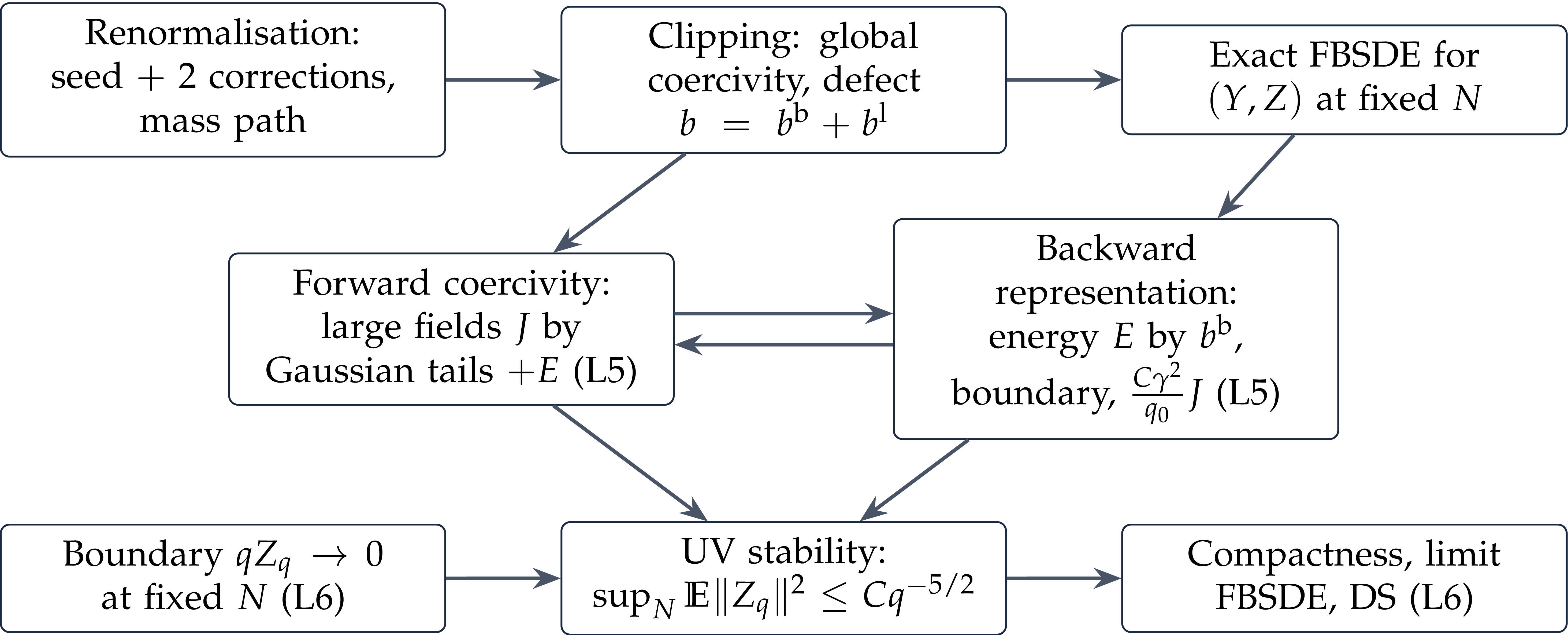
Summary of today, at every lattice:

• \(\mu_N\), \(M_q\) and a globally convex \(\bar{\Gamma}_q\), all deterministic;

• the exact FBSDE for \((Y, Z)\);

• a source whose bounded-field part is integrable (two steps), and whose large-field part is controlled by sixth powers of \(Y\) on large fields.

Next: estimates on \((Y, Z)\) uniform in \(N\).