A Constructive Introduction to Quantum Field Theory
\(\Phi^4_3\) on the torus II: a priori estimates
Massimiliano Gubinelli | University of Oxford
SISSA lectures, Lecture 5 — notes: Lecture 5, §§14–16
At each lattice \(N\), exactly (Lecture 4):
Inputs.
Coercivity: \(H_q (y) \asymp (K_q + \gamma y^2)^{- 1}\), \(\|H_q \|_{p \to p} \le (1 + \varepsilon_q) / q\), \(\varepsilon_q = C (g_q + g_q^2)\).
Source: \(\|b^{\text{b}}_q \|_{\infty} \le C \gamma^{7 / 2} q^{- 5 / 2}\), \(\|b^{\text{l}}_q (y)\|_2^2 \le C \gamma^4 q^{- 5} \|t_q (y)\|_6^6\).
Coordinates: \(K_q (Y_q + \varrho_q (Y_q)) + \frac{\gamma}{3} Y_q^3 = P_q\), \(\|D \varrho_q \|_{p \to p} \le \varepsilon_q\).
Goal
\(Z\) small and \(Y\) rarely at large fields, uniformly in \(N\). Neither equation can be estimated alone.
Usual (Ma–Yong): Lipschitz coefficients, Itô on \(\|Z\|^2\) and Gronwall; close on a short interval or under monotonicity.
Here: infinite interval, coefficients not uniformly Lipschitz, the coupling is not small. Instead we use structure:
the backward equation is linear in \(Z\) given \(Y\): a conditional representation with an explicit propagator;
the forward equation is, after subtracting the Gaussian part, a cubic elliptic equation at each resolution: coercive, estimated pathwise;
the two estimates are linked by two weighted energies with matched weights.
At fixed \(N, T\) all moments are finite (finite dimensions): used only to justify absorptions. Ma–Yong 1999
The energies
Lecture 5
Free field at resolution \(q\) driven by the same innovation:
Also \(P_q = W_q + \int (Y + Z)\). With \(V_q = Y_q + \varrho_q (Y_q) - X_q\) and \(F^Z_q = \int_{q_0}^q Z_s \mathrm{d} s\), the noise cancels:
At each \(q\): \((q - \Delta) V + \frac{\gamma}{3} (V + X - \varrho)^3 = f\), a nonlinear Helmholtz equation; \(X\) is a shift inside the cube.
The memory has coefficient one: \(\int_{q_0}^q V \approx qV\). It must be absorbed, not treated as forcing.
The backward equation enters only through \(F^Z = \int Z\). Pathwise.
| quantity | weight | reason |
| \(\|Z_q \|^2\) | \(q^{1 / 2}\) | Hardy: \(\int q^{- 3 / 2} \|F^Z \|^2 \le 16 \int q^{1 / 2} \|Z\|^2\) |
| \(\gamma \|t_q \|_6^6\) | \(q^{- 3 / 2}\) | \(q^{7 / 2} \|b^{\text{l}} \|^2 \le C \gamma^3 \cdot \gamma q^{- 3 / 2} \|t\|_6^6\) |
| \(\|b^{\text{l}}_q \|^2\) | \(q^{7 / 2}\) | propagator \(s / q\), \(\int_q^{\infty} s^{- 3 / 2} = 2 q^{- 1 / 2}\) |
Only thresholded sixth powers: unthresholded, \(\mathbb{E} \|X_q \|_6^6 \asymp q^{3 / 2}\) for \(2 q_0 \le q \lesssim N^2\), so \(\int \gamma q^{- 3 / 2} \mathbb{E} \|X_q \|_6^6 \approx \gamma N^2\) is not uniform in \(N\).
Lemma. For \(f\) on \([q_0, \infty)\), extended by zero to \((0, q_0)\),
Proof: \(q^{- 1} \int_0^q f = \int_0^1 f_{q \theta} \mathrm{d} \theta\), Minkowski; \(\int_0^1 \theta^{- 1 / 8} = \frac{8}{7}\), \((\int_0^1 \theta^{- 3 / 4})^2 = 16\).
The problem
\(\frac{8}{7} > 1\): the mass term alone (coefficient one) does not absorb the memory. The missing margin comes from the cube: at large fields it adds \(\frac{1}{4} q |w|^4\), and \(1 + \frac{1}{4} - \frac{8}{7} = \frac{3}{28} > 0\).
Forward coercivity
Lecture 5
Lemma.
and \(|t_q | \le \frac{32}{7} (|w_q | + | \xi_q |)\). Pathwise, uniform in \(\gamma\).
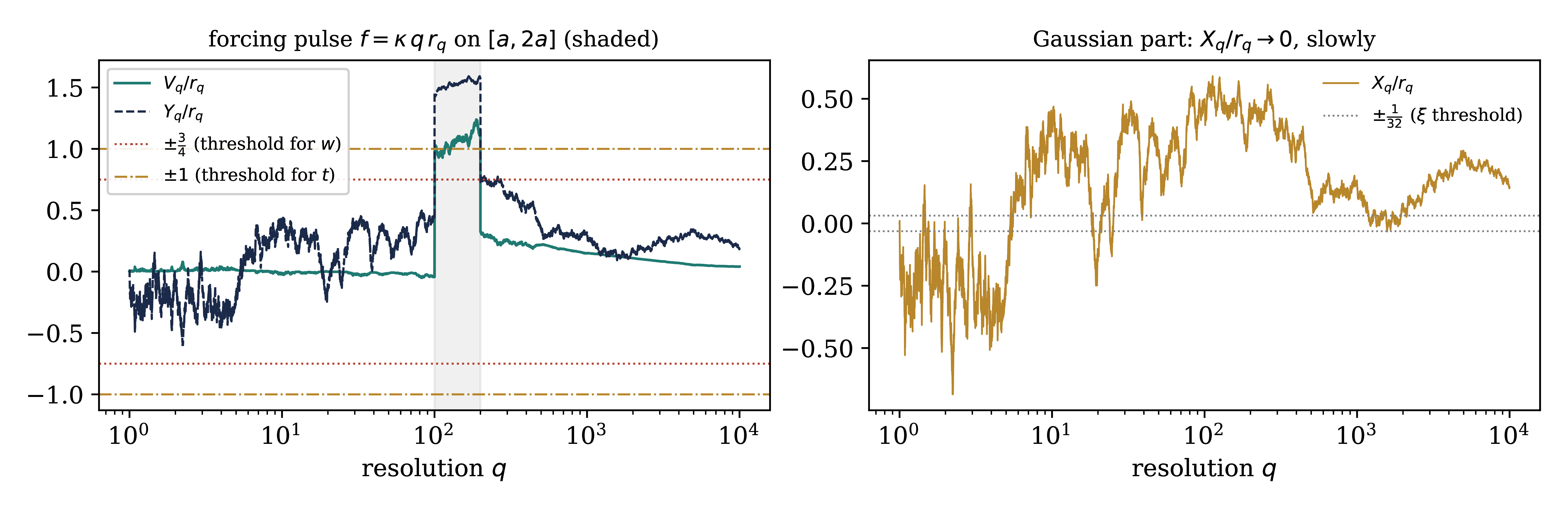
Forcing pulse \(f_q = \kappa \hspace{0.17em} qr_q \mathbb{1}_{[a, 2 a]} (q)\), \(\kappa\) of order one. Thresholds: \(\pm \frac{3}{4}\) for \(V_q / r_q\), \(\pm 1\) for \(Y_q / r_q\); the Gaussian part \(X_q / r_q\) on its own panel.
The pulse pushes \(V\) past \(\frac{3}{4} r\); the cube caps the excursion and brings it back. On this range \(|X_q | > r_q / 32\) most of the time: \(\xi_q\) is not rare until \(g_q\) is small (here \(q \gg 10^6\)). In this realisation the Gaussian part stays below the threshold, \(|X_q | / r_q < \frac{3}{4}\).
Where \(w \ne 0\): \(|v| = |w| + \frac{3}{4} r\), same sign.
Mass: \(qvw^3 = q|w|^4 + \frac{3}{4} qr |w|^3\).
Cube: \(|X| \le \frac{r}{32} + | \xi |\), so \(\text{sgn} (w) (v + X) \ge |w| + \frac{11}{16} r - | \xi |\); the cube is increasing, and
Large-field coercivity: a sixth power and a quarter of the mass.
Memory: \(|v - w| \le \frac{3}{4} r\), \(\int_{q_0}^q r \le \frac{2}{3} qr\): \(w^3 \hspace{-0.17em} \int v \le \frac{1}{2} qr|w|^3 + w^3 \hspace{-0.17em} \int w\); the first is absorbed by \(\frac{3}{4} qr |w|^3\).
Forcing: \(w^3 f \le \frac{\gamma}{48} w^6 + \frac{12}{\gamma} f^2\).
Multiply by \(q^{- 3 / 2}\), integrate, Hölder and Hardy: \(\int q^{- 3 / 2} w^3 \hspace{-0.17em} \int w \le \frac{8}{7} \int q^{- 1 / 2} w^4\), and \(\frac{5}{4} - \frac{8}{7} = \frac{3}{28}\).
For \(x, \rho \ge 0\):\(\frac{1}{4} x^3 + 64 \rho^3 - 3 x^2 \rho = \frac{1}{4} (x - 8 \rho)^2 (x + 4 \rho) \ge 0\), hence
With \(x = u + \frac{11}{16} r\): \(u^3 x^3 \ge u^6 + 3 (\tfrac{11}{16})^2 r^2 u^4\), \(\frac{3}{4} (\frac{11}{16})^2 = \frac{363}{1024} > \frac{1}{4}\), and \(\frac{65}{3} u^3 \rho^3 \le \frac{1}{6} u^6 + \frac{4225}{6} \rho^6\). So
What the scalar lemma says
The excess of the forecast over the threshold is controlled by how often the Gaussian field is large (known, \(N\)-independent) and by the backward forcing. No smallness of the coupling; pathwise.
Proposition.
New terms:
Laplacian: \(w^3 = \phi' (V)\), \(\phi\) convex, so \(\langle \phi' (V), - \Delta V \rangle = N^{- 1} \sum_{x \sim x'} (\phi' (V_x) - \phi' (V_{x'})) (V_x - V_{x'}) \ge 0\).
Coordinate correction: \(\varrho = \varrho^0 + \varrho^1\), \(\| \varrho^0 \|_{\infty} \le \varepsilon r\) (threshold shift; memory absorbed by the spare \(\frac{1}{4} qr |w|^3\)), \(\| \varrho^1 \|_j \le C \varepsilon (\|w\|_j +\| \xi \|_j)\) (memory absorbed by \(\frac{3}{28}\)). Operator bounds: \(\varrho\) is nonlocal but small.
Backward forcing: \(\gamma^{- 1} \int q^{- 3 / 2} \|F^Z \|^2 \le 16 E_T\).
Gaussian tails: \(\text{Var} X_q (x) \lesssim \sqrt{q}\) vs threshold \(\frac{1}{32} (q / \gamma)^{1 / 2}\): \(| \| \xi_q \|_j^j |_p \le C_j p^{j / 2} q^{j / 4} \mathrm{e}^{- c \sqrt{q} / (p \gamma)}\).
\(X\) is Gaussian under the interacting measure: no information on the interacting field is used.
Backward feedback and closure
Lecture 5
Propagator: \(\partial_s \mathscr{P}_{q, s} = \mathscr{P}_{q, s} H_s (Y_s)\), \(\mathscr{P}_{q, q} = I\), and by (A)
Lemma.
Proof: \(\mathrm{d}_s (\mathscr{P}_{q, s} Z_s) = - \mathscr{P}_{q, s} b_s \mathrm{d} s + \mathscr{P}_{q, s} \Xi_s \mathrm{d} W_s\), a true martingale at fixed \(N\).
\(Z\) = expected source on the unresolved scales, transported back, plus the boundary error. Compare \(F_t =\mathbb{E}_t [F_T]\) in Lecture 3: here the source is the defect.
Bounded fields (two correction steps!):
Boundary: \(q \|Z^{\text{t}}_q \| \le L_0 \mathbb{E}_q \|TZ_T \|\), contributing \(\frac{2 L_0^2}{\gamma q_0^{1 / 2}} \delta_{N, T, p}\), \(\delta_{N, T, p} = \|TZ_T \|^2_{L^{2 p} (\mathbb{P}; L^2)}\).
Large fields: \(A^{\text{l}} = \int s^{7 / 2} \|b^{\text{l}}_s \|^2 \le C \gamma^3 J_T\); Cauchy–Schwarz and Jensen,
This is how the clipping error is controlled
\(b^{\text{l}}\) is not small, but it enters the backward energy only through the large-field action \(J_T\), with the small factor \(\gamma^2 / q_0\).
Theorem.
\(x = \|E_T \|_p\), \(y = \|J_T \|_p\):\(y \le A_0 (C \gamma^3 p^5 + x)\), \(x \le B_0 + B_1 \delta + \eta y\), \(\eta = C \gamma^2 / q_0 = Cg_{q_0}^2\). Choose \(A_0 \eta \le \frac{1}{2}\); \(y < \infty\) at fixed \(N, T\), absorb.
The smallness is in the feedback, independent of \(p\): one \(q_0\) for all \(p\); the growth \(p^5\) is inherited from \(G_T\).
Once the boundary term is removed (Lecture 6):
and \(\mathbb{E} \exp \{c (E_{\infty} + J_{\infty})^{1 / 5} \} < \infty\).
The approximate forecast differs from the exact one by \(O (q^{- 5 / 4})\) in \(L^2 (\mathbb{P}; L^2)\) (root mean square), uniformly in the lattice.
\(H_q Z_q = O (q^{- 9 / 4})\) in \(L^2 (\mathbb{P}; L^2)\): up to an integrable drift, the forward equation is the explicit SDE \(\mathrm{d} Y = b (Y) \mathrm{d} q + H (Y) \mathrm{d} W\).
Comparison with Boué–Dupuis (Lecture 3)
There: drift \(u = - 4 \lambda \dot{Q}^{1 / 2} : X^3 : + r\) (\(\lambda \int : \varphi^4\): of Lecture 3). Here: \(\bar{\Gamma}\) does all such changes of variables at once in the forecast coordinate; \(Z\) plays the role of \(r\). Coercivity of the quartic: pathwise in the forward equation; the remainder: in expectation through the backward one.
Barashkov–G. 2020
