the boundary term vanishes: \(TZ_T \to 0\) at
fixed \(N\);
uniform energy bounds \(\Rightarrow\)
compactness of processes and measures;
identify the limit: coefficients, noise, equations.
The subtle point
Convergence of the fields does not pass an FBSDE to the limit: the
backward martingale could acquire extra noise. The
statistical meaning of the backward variable saves us.
The boundary at infinite
resolution
Lecture 7
The boundary lemma
\(\bar{\Gamma}_q\) was built to converge to the
bare action: \(\mu_q \to \mu_N\), \(\Theta_q
\to 0\), corrections integrated from \(q =
\infty\).
compare \(\mathbb{E}_q G\) with the
observed \(G^0_q = DV_N
(\Phi_q)\): \(\|\mathbb{E}_q G - G\| \le 2 \|G
- G^0_q \|\).
No uniform estimate, no posterior concentration.
UV stability
Let \(T \to \infty\) at fixed \(N\)
(paths and \(\nu_N\) do not depend on \(T\);
monotone convergence; \(\delta_{N, T, p} \to 0\)).
Only then take \(\sup_N\).
Theorem.
(UV
stability) For \(q_0 = q_0
(\gamma)\) large,
\(C_{N, p}\) diverges with \(N\):
never take \(\sup_N\) of \(C_{N,
p} / T\).
The force: \(F_q =\mathbb{E}_q [- DV_N
(\Phi_{\infty})] = K_q Z_q - D \bar{\Gamma}_q (Y_q)\), the
explicit force at the approximate forecast, corrected by \(K_q Z_q\).
Compactness
Lecture 7
Suprema by a maximum principle
Embed by cells \(\square_x\): \(\iota_N
: H_N \to H = L^2 (\mathbb{T}^3)\) isometric, \(j_N
= \iota_N^{\ast}\).
At frozen \(q\): \(K_q U +
\frac{\gamma}{3} (U + d)^3 = f\). Constants are super- and
subsolutions: lattice maximum principle.
The weight \(q^{- \varpi}\) absorbs the
memory: \(q^{- 1 - \varpi} \int_{q_0}^q s^{\varpi}
\le (1 + \varpi)^{- 1}\).
Finite-resolution suprema have all moments uniformly in \(N\);
the terminal field is a distribution.
Regularity and the terminal field
Space. \(K_q V_q = f_q\) with \(\mathbb{E}
\int_I \|f\|_2^2 \le C_I\) (energies), so \(V \in
L^2 (I ; H^1)\); \(Y = V + X - \varrho
(Y)\) has the regularity of the free field: \(H^{\sigma}\),
\(\sigma < \frac{1}{2}\), in space; \(H^{\theta}\),
\(\theta < \frac{1}{2}\), in scale; tight in
space–time \(L^p\) (and in \(C
(I ; H)\): \(C^{1 / 4}\) Hölder bound
\(+\) uniform Fourier tails).
Terminal field. \(H_q^2 \le \frac{C}{q}
C_q\) gives, for \(\frac{1}{2} < s <
\frac{3}{2}\),
\(\displaystyle \int_Q^{\infty} \|(1 - \Delta)^{- s / 2} H_q
\|_{\text{HS}}^2 \mathrm{d} q \le
C \int_Q^{\infty} \frac{1}{q}
\sum_k \frac{(1 + |k|^2)^{- s}}{q + c |k|^2}
\mathrm{d} q \le C_s Q^{-
(s - \frac{1}{2})},\)
and the drifts have squared tails \(O (Q^{- 3})\),
\(O (Q^{- 5 / 2})\), \(O (Q^{- 3 /
2})\). Doob:
Corollary.
\(\nu_N\) is tight in
\(H^{- s} (\mathbb{T}^3)\) for every \(s
> \frac{1}{2}\), with all moments uniformly in \(N\).
(Threshold of the free field in \(d = 3\).)
Identifying the limit
Lecture 7
The deterministic coefficients
Uniform bounds do not identify a limit: a weakly convergent vertex
cannot in general be contracted against a varying covariance. Three
tools:
Weak vertex measures: bounded rooted norms \(\Rightarrow\) signed measures, weakly compact; the
centred kernel in a first-moment topology. The limits solve the
same fixed point, unique in its ball: the whole sequence
converges.
Contraction against a moving covariance: rows of
the inverses are Hölder \(+\) HS
convergence \(\Rightarrow\) \((H^N)^2
\to H^2\) uniformly; weak vertices can be contracted.
Hence \(H^N_q (Y^N_q) \to H_q (Y_q)\) in \(L^2 (I ; \text{HS})\) and \(b^N_q (Y^N_q)
\to b_q (Y_q)\) in \(L^2 (I ; H)\).
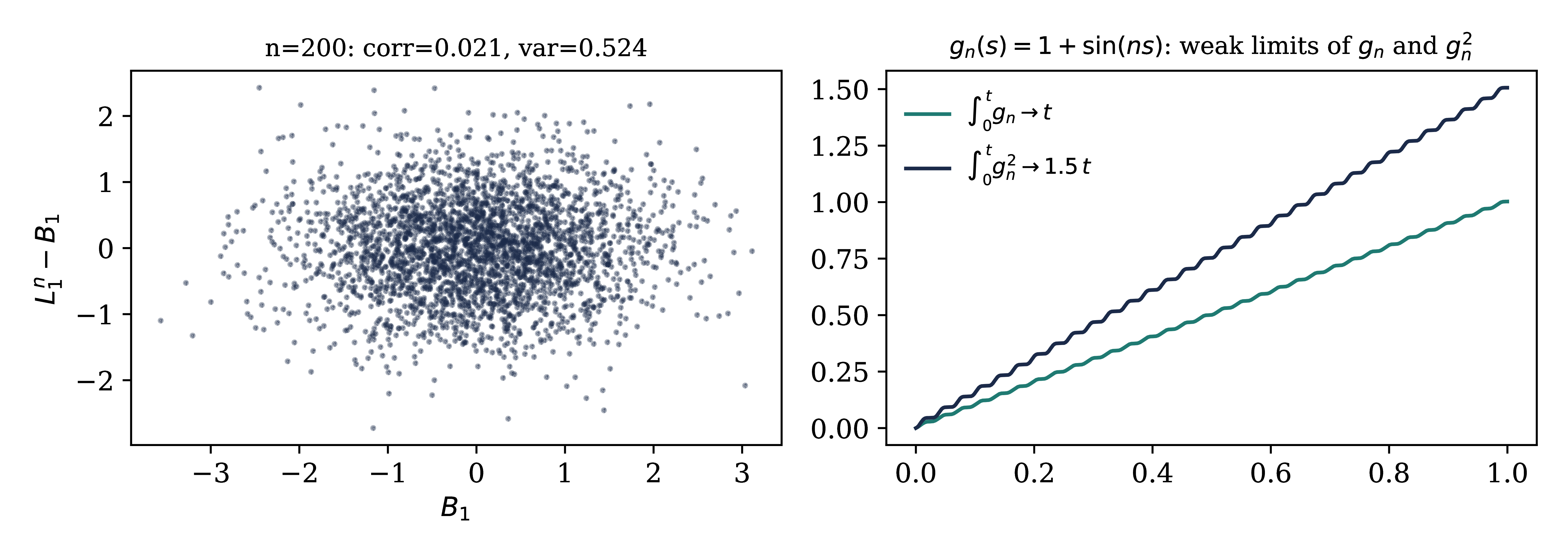
Left: \((B_1, L^n_1 - B_1)\), \(n =
200\): correlation \(\approx 0\), variance
of the gap \(\approx \frac{1}{2}\) — the
residual does not vanish and is orthogonal to \(B\).
Right: \(\int_0^t g_n \to t\) but \(\int_0^t
g_n^2 \to \frac{3}{2} t\).
A limiting FBSDE obtained this way would carry an extra
martingale orthogonal to the driving noise. We need
strong compactness of the backward integrand \(\Xi = \text{Cov} - H (Y)\).
The Riccati equation of the posterior covariance
Lemma.
\(\text{Cov}_q = D^2
\mathcal{K}_q (P_q) \ge 0\) and
Lecture 4: conditional variance is resolved at rate \(\text{Cov}_t
\dot{\mathscr{R}}_t \text{Cov}_t\); here \(\partial_q
\mathscr{R} = 1\).
\(\langle f, \text{Cov}_q f \rangle \ge 0\): a
nonnegative supermartingale, initial value \(\text{Var}_{\nu_N} \langle \Phi_{\infty}, f
\rangle\) bounded uniformly (uniform moments, Corollary).
Stop at level \(K\): decreasing part and
bracket have bounded expectations \(\Rightarrow\)
time regularity \(W^{a, 1}\), \(a
< \frac{1}{2}\) \(\Rightarrow\) strong
compactness of each finite block.
\(\Rightarrow\) \(\text{Cov}^N\)
tight in strong \(L^2 (I ; \text{HS})\); brackets
\(\int \text{CovCov}^{\ast}\) and covariations
with \(W\) converge.
Identification of the martingales
On a common filtered space (Skorokhod), along a subsequence:
\(\psi\) is a continuous square-integrable
martingale for the joint filtration; its bracket and its
covariation with \(W\) are those of \(\int \text{Cov} \hspace{0.17em} \mathrm{d} W\);
so \(\psi - \int \text{Cov} \hspace{0.17em}
\mathrm{d} W\) has zero bracket and vanishes: no
extra martingale;
same for the forward equation, and \(X = \int C
\hspace{0.17em} \mathrm{d} W\) with the
same \(W\) (needed to pass
the thresholded energies).
\(\displaystyle \begin{aligned}
Y_q & = \int_{q_0}^q [b (Y) + H (Y)
Z] \mathrm{d} s + \int_{q_0}^q H (Y)
\hspace{0.17em} \mathrm{d}
W,\\
Z_q & = - \int_{q_0}^q [b (Y) + H (Y) Z] \mathrm{d} s +
\int_{q_0}^q \Xi
\hspace{0.17em} \mathrm{d} W, \qquad X_q =
\int_{q_0}^q C_s \hspace{0.17em}
\mathrm{d} W_s .
\end{aligned}\)
The result (I): convergence and the limiting FBSDE
Theorem.
(subsequential
construction) For \(\lambda
> 0\), \(q_0\) large, along a subsequence
of lattices:
\((Y^N, Z^N, \psi^N, X^N)\) converge in
\(C (I ; H)\), \(W^N\)
in \(C (I ; H^{- r})\), \(r >
\frac{3}{2}\), \((\text{Cov}^N,
\Xi^N)\) in strong \(L^2 (I ;
\text{HS})\), jointly, a.s. on a new space;
the limit solves the FBSDE on \([q_0,
\infty)\) with the continuum coefficients \(b,
H\) (unique in their ball), an \(H\)-cylindrical
Brownian motion obtained as the limit of the lattice
innovations, \(\text{Cov} = H (Y) + \Xi \ge
0\), and \(\mathbb{E} \|Z_q \|^2 \le Cq^{- 5
/ 2}\);
\(\psi^N\) is tight in \(C (I ;
H)\) because its brackets \(\int \text{Cov}^N
\text{Cov}^{N \ast}\) are tight and its Fourier tails are
uniformly small.
The result (II): the terminal law
Theorem.
(subsequential
construction, continued)
\(Y_q \to \Phi\) in \(H^{-
s}\), \(s > \frac{1}{2}\), a.s. and
in mean square; \(\text{Law} (\Phi) = \nu\)
is the weak limit of \(\nu_N\), and \(\langle Y_q + Z_q, h \rangle =\mathbb{E} [\langle \Phi,
h \rangle
\hspace{0.17em} | \hspace{0.17em}
\mathcal{F}_q]\);
the limiting thresholded energies (built with \(X =
\int C \hspace{0.17em} \mathrm{d} W\)) obey the bounds of
UV stability.
The posterior structure survives: \(\psi = Y + Z\)
is a closed observable, \(Y\) is
computed from the explicit action, \(Z\) is small
at high resolution.
\(\displaystyle \lim_N \mathbb{E} [G (\iota_N \Phi^N_{\infty})
\langle \mu_N \Phi^N_{\infty} +
\lambda (\Phi^N_{\infty})^3, j_N h
\rangle] =\mathbb{E}_{\nu} [D_h G (\Phi) -
G (\Phi) \langle \Phi,
(q_0 - \Delta) h \rangle] .\)
Proof: lattice Gaussian integration by parts in \(\mathrm{e}^{-
V_N - \frac{1}{2} \langle \varphi, K_{q_0} \varphi \rangle}\);
\(K_{q_0} j_N h = j_N (q_0 - \Delta^{\text{tr}}_N)
h\); tightness and uniform moments.
The terminal case of the DS equations of Lecture 4.
The renormalised cube \(\mu_N \Phi + \lambda
\Phi^3\) is identified only tested in
expectation, not as a random distribution.
Consistent with the expectation (Lecture 4) that the limiting
force is an observable without terminal representative; this is
not proved.
At every finite resolution the force is explicit: \(F_q
= K_q Z_q - D \bar{\Gamma}_q (Y_q)\).
What is not proved
Uniqueness of the limit, of the FBSDE,
independence of the regularisation.
Small mass / strong coupling: the construction
needs \(\gamma q_0^{- 1 / 2}\) small, i.e.
weak coupling \(\lambda / m \ll 1\). Removing
it needs a priori estimates without the small feedback \(\gamma^2 / q_0\), and a coefficient construction
outside the perturbative ball.
Axioms: reflection positivity holds on the
lattice (lattice and mid-lattice planes) and passes to \(\nu\) for every coordinate reflection (standard;
exercise); rotation invariance and clustering need infinite
volume.
Infinite volume: the force and its Burgers flow
are intensive; estimates must be made local. Uniform-in-volume
coefficient bounds and local energy moments are open; retaining
the full FBSDE also needs control of the noise from
infinity in the nonlocal \(\Xi\).
Summary of the course
Wightman \(\to\) Euclidean (L1) \(\to\)
free field (L2) \(\to\) stochastic quantisation,
scale decomposition (L3) \(\to\) Polchinski,
FBSDE, variational problem (L4) \(\to\) \(\Phi^4_3\) through the FBSDE in forecast coordinates
(L5–7).
Lecture 4 (formal)
Lectures 5–7
in the limit
forecast \(\psi_t =\mathbb{E}_t
\Phi_T\)
\(\psi = Y + Z\)
closed martingale
response \(H_t =
\text{Cov}_t\)
\(\text{Cov} = H (Y) + \Xi\)
strong \(L^2 (\text{HS})\),
Riccati
\(\Gamma_t\), Wetterich
\(\bar{\Gamma}_q\) explicit, defect
\(e\)
deterministic coefficients
force \(F_t\)
\(K_q Z_q - D \bar{\Gamma}_q
(Y_q)\)
observable at finite \(q\)
DS equation
integration by parts
tested in expectation
UV stability \(=\) an explicit
action predicts the conditional mean up to an error that is small at
high resolution.