Constructive quantum field theory — Lecture 4 (notes)

Introduction

Lecture 3 formulated a programme (Figure 5.1 and the remark following it): solve the FBSDE

with a renormalised interaction \(V_T\), with estimates uniform in the ultraviolet cutoff, and take the limit. For \(\Phi^4_3\) the force \(F_t\) is not expected to converge to an integrable terminal value, and the naive estimates of the force diverge (Section 9.2). In these three lectures we carry out a version of the programme on the unit torus \(\mathbb{T}^3\), for a large mass. The guiding principle is the one of Section 6: do not estimate \(\Phi\) and \(F\) directly, but pass to the forecast coordinate, in which the forward equation has no drift and the tree diagrams have been integrated exactly.

The argument has three parts, one per lecture.

1. Deterministic renormalisation (this lecture). Construct an explicit approximate effective average action \(\bar{\Gamma}_q\) and a counterterm, by a finite number of steps of the Wetterich flow, and estimate its defect.

2. A priori estimates (Lecture 5). Write the exact FBSDE in the coordinates of \(\bar{\Gamma}_q\), and estimate the forward and the backward equation together, uniformly in the lattice.

3. Removing the cutoffs (Lecture 6). Remove the upper scale at fixed lattice, then the lattice, and identify the limiting FBSDE and its terminal law.

The emphasis is on the structure of the argument. We give complete proofs of the identities and of the scalar models of the estimates, and only describe the tensor estimates on the lattice. The lectures follow the course notes [FBSDE26], where all the estimates are proved. The point of view is that of [BCG26]; for other constructions of \(\Phi^4_3\) see [GJ73, FO76, BFS83, BG20, GH21].

What is proved.

11The problem and the exact FBSDE

11.1Lattice, scales and notation

Let \(N\) be an odd integer and \(\Lambda_N = (N^{- 1} \mathbb{Z}/\mathbb{Z})^3\) the periodic lattice of mesh \(N^{- 1}\) in the unit torus. Let \(H_N =\mathbb{R}^{\Lambda_N}\) with

so that the volume is \(1\) and integrals approximate continuum integrals. The nearest-neighbour Laplacian is \(\Delta_N u (x) = N^2 \sum_{i = 1}^3 [u (x + e_i / N) + u (x - e_i / N) - 2 u (x)]\); we usually drop the index \(N\). A kernel \(C (x, z)\) acts by \(Cu (x) = \int C (x, z) u (z) \mathrm{d} z\), so the identity has kernel \(N^3 \mathbb{1}_{x = z}\), and

\(M_f\) is multiplication by \(f\), and \(K + \gamma y^2\) means \(K + \gamma M_{y^2}\). For a functional \(F\) on \(H_N\), \(DF\), \(D^2 F\), \(D^k F\) are its gradient and derivatives, as in Lecture 3. \(\|u\|_p\) is the \(L^p\) norm for the measure \(\int\).

The resolution parameter.

It is convenient to parametrise the resolution by the squared regulator mass

Set

In the notation of Lecture 3, with \(T = \infty\) and using \(q\) instead of \(t\) as the resolution variable (so \(\dot{Q}\) now means \(\partial_q Q_q\)),

So \(C_q\) is the covariance of the scales not yet resolved, and \(K_q = S_q^{- 1}\) is the precision of the posterior at resolution \(q\) under the free prior \(\mu^C\). The main properties of \(C_q\) are elementary.

Lemma 11.1. (Free resolvents) For \(q \geq 1\), uniformly in \(N\): \(C_q\) has a nonnegative kernel, \(C_q \mathbb{1} = q^{- 1} \mathbb{1}\), \(\|C_q \|_{p \to p} = q^{- 1}\) for \(1 \le p \le \infty\), and

For \(y \in H_N\) and \(\gamma > 0\), the killed resolvent \(G_q (y) = (K_q + \gamma y^2)^{- 1}\) satisfies \(0 \le G_q (y) (x, z) \le C_q (x, z)\).

Proof. \(C_q = \int_0^{\infty} \mathrm{e}^{- qs} \mathrm{e}^{s \Delta} \mathrm{d} s\) and \(\mathrm{e}^{s \Delta}\) is the transition kernel of the lattice random walk. This gives positivity and the row sums. Killing the walk at rate \(\gamma y^2\) gives the comparison for \(G_q\). The symbol of \(- \Delta_N\) is comparable to \(|k|^2\) on the centred frequency cube \(n \in \{- \frac{N - 1}{2}, \ldots, \frac{N - 1}{2} \}^3\) (symbol \(4 N^2 \sum_i \sin^2 (\pi n_i / N)\), with \(k = 2 \pi n\)), and \(\sum_k (q + |k|^2)^{- 2} \le C \int_{\mathbb{R}^3} (q + |k|^2)^{- 2} \mathrm{d} k = Cq^{- 1 / 2}\). Counting the \(N^3\) modes gives the other bounds.\(\Box\)

The bubble \(a_2 (q)\) is the coincident-point variance of the shell at resolution \(q\): \(\partial_q \text{Var} (X_q (x)) = a_2 (q)\) for the free field at resolution \(q\), and \(\int_{q_0}^{\infty} a_2 = \text{Tr} C_{q_0} \asymp N\) is the divergent variance of the lattice field.

11.2The cutoff measure and the goal

Fix \(\lambda > 0\) and put \(\gamma := 3 \lambda\) (not to be confused with the counterterm \(\gamma_T\) of Lecture 3). The interaction and the lattice measure are

where \(\mu^C\) is the centred Gaussian measure with covariance \(C = C_{q_0}\) on \(H_N\), and \(\mu_N \in \mathbb{R}\) is a mass counterterm to be chosen. With this normalisation \(D^2 U (y) = \gamma M_{y^2}\). In Lecture 3 we wrote the interaction as \(\lambda \int H_4 (\varphi ; c_T) + \gamma_T \int H_2 (\varphi ; c_T)\); the Wick ordering is now part of \(\mu_N\), and the coupling is rescaled by \(4\). For every real \(\mu_N\), \(\nu_N\) is a probability measure with all moments, since the quartic term dominates.

Theorem 11.2. (Main result, informal [FBSDE26]) Let \(\lambda > 0\) and let \(q_0\) be large enough, depending on \(\lambda\). There are explicit \(\mu_N\), with \(\mu_N = - 3 \lambda \text{Tr} C + O (\log N)\), such that:

The bounds that prove (a) and (b) are uniform in \(N\): this is UV stability. They are bounds on the error \(Z\) of an approximate forecast, defined below. We now set up the exact FBSDE at fixed \(N\).

11.3The Polchinski process as a posterior

At a fixed lattice everything can be realised by a simple statistical experiment. Let \(\Phi_{\infty} \sim \nu_N\), and let \(B\) be an independent Brownian motion on \(H_N\), \(\mathbb{E} \langle B_t, u \rangle \langle B_s, v \rangle = (t \wedge s) \langle u, v \rangle\). We observe

with the filtration \(\mathcal{F}_q\) generated by \((P_s)_{s \le q}\) (completed), and \(\mathbb{E}_q =\mathbb{E}[\hspace{0.17em} \cdot \hspace{0.17em} |\mathcal{F}_q]\). Let

Proposition 11.3. (Posterior, forecast and innovation) At every fixed \(N\):

Proof. (a) Conditionally on \(\Phi_{\infty} = \varphi\), the density of the observed path on \([q_0, q]\) with respect to the law of \(B\) is \(\exp \{\langle P_q, \varphi \rangle - \frac{q - q_0}{2} \| \varphi \|^2 \}\) (Girsanov, or a direct computation on finitely many increments). Bayes' formula gives \(\nu_{q, P_q}\), and differentiating \(\mathcal{K}_q\) in \(p\) gives the conditional moments. Positivity of \(\text{Cov}_q\) holds because \(\nu_{q, p}\) has a positive density. (b) For \(s < q\), \(\mathbb{E}_s [P_q - P_s] = (q - s) \psi_s\) since \(B\) has independent increments, and \(\mathbb{E}_s \int_s^q \psi_u \mathrm{d} u = (q - s) \psi_s\) since \(\psi\) is a martingale. So \(W\) is a continuous martingale with \(\mathrm{d} \langle W, W \rangle_q = I \hspace{0.17em} \mathrm{d} q\), and Lévy's theorem applies. (c) \(\partial_q \mathcal{K}= - \frac{1}{2} \mathbb{E}_{\nu_{q, p}} \| \varphi \|^2\) and \(\text{Tr} D^2 \mathcal{K}=\mathbb{E}_{\nu_{q, p}} \| \varphi \|^2 - \|D\mathcal{K}\|^2\). Differentiating (c) in \(p\) and applying Itô's formula along \(\mathrm{d} P = D\mathcal{K} (P) \mathrm{d} q + \mathrm{d} W\), the drift of \(D\mathcal{K}_q (P_q)\) cancels, which gives \(\mathrm{d} \psi = \text{Cov} \hspace{0.17em} \mathrm{d} W\).\(\Box\)

The observation \(P_q\) is not yet the field of Lecture 3. The posterior (11.6) is \(\nu_N\) tilted by a Gaussian factor of precision \(q - q_0\): the remaining randomness has precision \(K_{q_0} + (q - q_0) = K_q\). This suggests the following.

Proposition 11.4. (The Polchinski process) Let \(\Phi_q := C_q P_q\) and \(F_q := K_q (\psi_q - \Phi_q)\). Then

This is the FBSDE (5.7) of Lecture 3 for the profile (11.2): \(\Phi\) is the interacting field at resolution \(q\), \(F\) the effective force, \(\psi\) the forecast of Proposition 6.1, and \(\text{Cov}_q = H^{\text{ex}}_q (\psi_q)\) (Proposition 11.5) is the response of Proposition 6.3. Under \(\nu_N = \mu^C\) one has \(F = 0\), \(\Phi_q = \psi_q\), and \(\Phi_q\) is the Gaussian field \(X_q\) of Proposition 4.2, with law \(\mu^{Q_q}\).

Proof. \(\mathrm{d} \Phi_q = - C_q^2 P_q \hspace{0.17em} \mathrm{d} q + C_q (\psi_q \mathrm{d} q + \mathrm{d} W_q) = C_q (\psi_q - \Phi_q) \mathrm{d} q + C_q \mathrm{d} W_q\), which is the first identity. For the second, integrate by parts in the density of \(\nu_{q, p}\) with respect to Lebesgue measure, \(\exp \{\langle p, \varphi \rangle - \frac{1}{2} \langle \varphi, K_q \varphi \rangle - V_N (\varphi)\}\): there is no boundary term, and

At \(p = P_q = K_q \Phi_q\) this reads \(K_q (\psi_q - \Phi_q) =\mathbb{E}_q [- DV_N (\Phi_{\infty})]\). In the Gaussian case the posterior is \(\mu^{C_q} (\cdot - C_q P_q)\), so \(\psi = \Phi\) and \(\Phi_{\infty} - \Phi_q\) is independent of \(\mathcal{F}_q\) with covariance \(C_q\). Hence \(\Phi_q\) is a Gaussian martingale with covariance \(C - C_q = Q_q\). In general both the law of \((\Phi_{\infty}, (\Phi_q)_q)\) here and the law of \((X_{\infty}, (X_q)_q)\) under the measure \(\mathbb{P}\) of Proposition 5.2 are the Gaussian law tilted by the same function \(\mathrm{e}^{- V_N} /\mathcal{Z}_N\) of the terminal field, so they coincide. Since \(P_q = K_q \Phi_q\), the filtration \((\mathcal{F}_q)\) is also the one generated by \(\Phi\).\(\Box\)

So at a fixed lattice the FBSDE of Lecture 3 is a theorem, with a Brownian motion \(W\) which is explicitly the innovation of a filtering problem. All objects of Section 6 have a statistical meaning:

The observations need no ultraviolet regularity: \(P_q\) is defined for every \(q\), with terminal resolution \(\infty\) at fixed \(N\). The lattice is the only ultraviolet cutoff, and \(\Phi_q \to \Phi_{\infty}\) as \(q \to \infty\) (Lemma 17.1).

11.4The Wetterich formulation

Let \(\Psi_q := \mathcal{K}_q^{\ast}\) be the Legendre transform of the log-partition function and

Comparing with (6.11), and using \(S_q^{- 1} = K_q\), \(\Gamma_q\) is, up to a function of \(q\) alone, the \(\Gamma_t\) of Lecture 3: \(\Gamma_q + \frac{1}{2} \langle y, K_{q_0} y \rangle\) is the effective average action with the regulator \(\mathscr{R}_q = q - q_0\) (Exercise 11.1). The coordinate identity \(P_q = D \Psi_q (\psi_q)\) reads

which is (6.5) with \(\mathscr{F}_q = D \Gamma_q\).

Proposition 11.5. (Wetterich equation with a mass regulator) At fixed \(N\), \(\Gamma_q\) is smooth and strictly convex after adding \(\frac{1}{2} \langle y, K_q y \rangle\), and

Proof. \(\mathcal{K}_q\) is smooth, strictly convex (its Hessian is a covariance) and superlinear (the posterior has full support), so \(\Psi_q\) is smooth and \(D^2 \Psi_q (D\mathcal{K}(p)) = (D^2 \mathcal{K}(p))^{- 1}\). By the envelope theorem at fixed \(y\) and Proposition 11.3(c), \(\partial_q \Psi_q (y) = - \partial_q \mathcal{K}_q (p) = \frac{1}{2} \text{Tr} D^2 \mathcal{K}_q (p) + \frac{1}{2} \|y\|^2\), with \(p = D \Psi_q (y)\). Subtract \(\partial_q \frac{1}{2} \langle y, K_q y \rangle = \frac{1}{2} \|y\|^2\).\(\Box\)

This is (6.12) with \(\partial_q \mathscr{R} = 1\), up to the constant \(- \frac{1}{2} \text{Tr} C_q\) (which is infinite in the continuum and irrelevant here). It is an identity about the unknown measure \(\nu_N\), not a construction: to use it we would need estimates on \(\Gamma_q\), which is what we want to prove. Lecture 3 suggests the strategy: since the FBSDE in forecast coordinates is

an approximate effective action gives approximate forecast coordinates, and the error should be governed by how badly the approximate action fails to solve (11.13).

11.5Approximate forecast and error

Let \(\bar{\Gamma}_q\) be an even functional on \(H_N\), smooth in \(q\) and \(y\), such that \(\bar{\Psi}_q (y) = \frac{1}{2} \langle y, K_q y \rangle + \bar{\Gamma}_q (y)\) is uniformly convex, \(D^2 \bar{\Psi}_q \ge \underline{c}_q I\) with \(\underline{c}_q > 0\). Let \(\bar{\mathcal{K}}_q = \bar{\Psi}_q^{\ast}\) and define the approximate response, the defect and its drift

The subtraction of \(H_q (0)\) only removes a function of \(q\). Define the approximate forecast and the error

Equivalently \(Y_q\) solves the approximate coordinate equation \(K_q \Phi_q = K_q Y_q + D \bar{\Gamma}_q (Y_q)\), i.e. (11.12) with \(\bar{\Gamma}\) in place of \(\Gamma\). If \(\bar{\Gamma} = \Gamma\) then \(Y = \psi\), \(Z = 0\), and \(e\) depends only on \(q\), so \(b = 0\).

Theorem 11.6. (The FBSDE in approximate forecast coordinates) At every fixed \(N\),

with \(Y_{q_0} = Z_{q_0} = 0\), and \(Y + Z = \psi\) is the martingale \(\int \text{Cov} \hspace{0.17em} \mathrm{d} W\).

Proof. By the Legendre identities \(\partial_q \bar{\mathcal{K}}_q (p) = - \partial_q \bar{\Psi}_q (y) = - \frac{1}{2} \|y\|^2 - \partial_q \bar{\Gamma}_q (y)\) and \(D^2 \bar{\mathcal{K}}_q (p) = H_q (y)\) at \(y = D \bar{\mathcal{K}}_q (p)\). Hence

Differentiate in \(p\): \(\partial_q D \bar{\mathcal{K}} + \frac{1}{2} \text{Tr} D^2 (D \bar{\mathcal{K}}) + D^2 \bar{\mathcal{K}} \hspace{0.17em} D \bar{\mathcal{K}} = - H \hspace{0.17em} De = b\). Now apply Itô's formula to \(Y_q = D \bar{\mathcal{K}}_q (P_q)\) along \(\mathrm{d} P = \psi \hspace{0.17em} \mathrm{d} q + \mathrm{d} W\):

which is the first equation, since \(\psi - Y = Z\). The second is \(\mathrm{d} Z = \mathrm{d} \psi - \mathrm{d} Y\) and (11.8). At \(q = q_0\), \(P_{q_0} = 0\) and evenness give \(Y_{q_0} = 0 = \psi_{q_0}\).\(\Box\)

Reading (11.16).

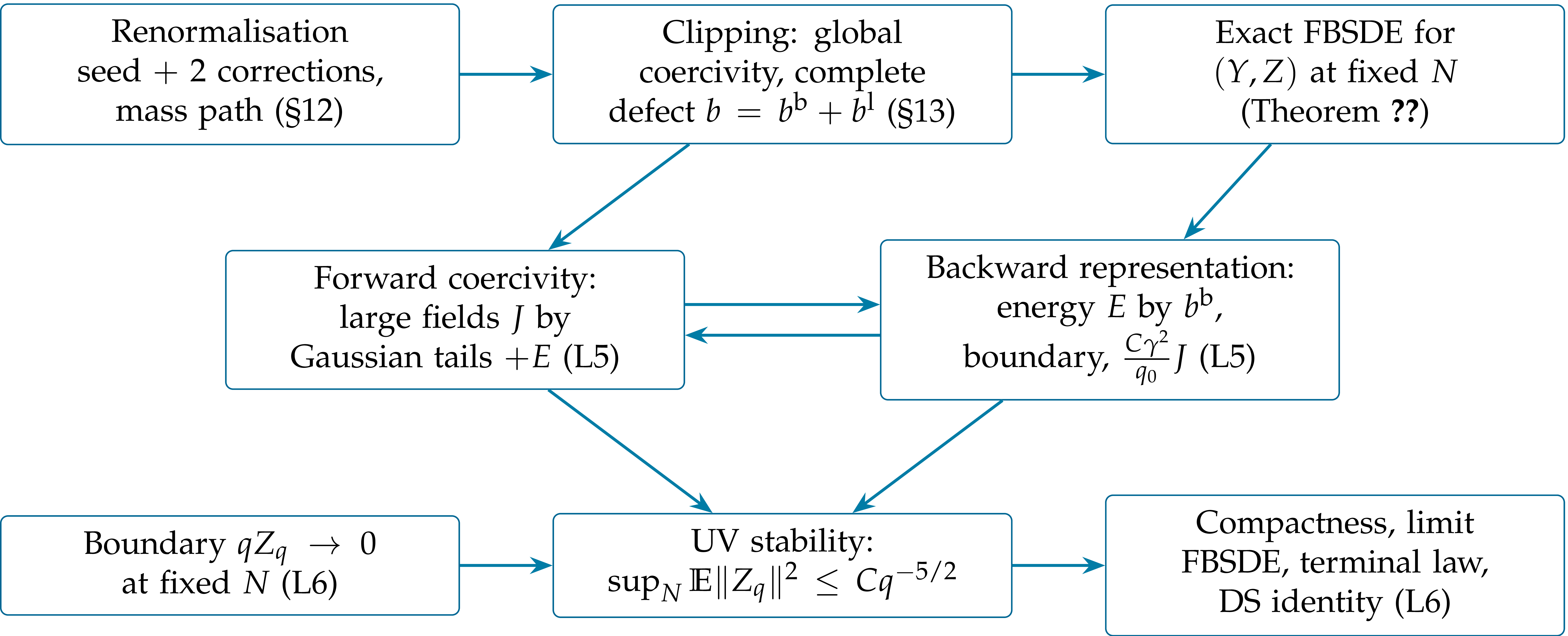
For this we need: (i) a defect \(e\) whose gradient is integrable against the backward propagator, which is a deterministic renormalisation problem (Section 12); (ii) global coercivity of \(\bar{\Gamma}\), so that \(H_q (y)\) is a good noise coefficient for all fields (Section 13); (iii) a priori estimates for the coupled system (Lecture 5). Figure 11.1 summarises the logic of the three lectures.

Figure 11.1. The structure of the construction. The two arrows between the forward and backward estimates form the closed loop of Lecture 5: neither estimate closes on its own.

Exercises

12Renormalisation: why two of them

We now construct \(\bar{\Gamma}_q\) on bounded fields. This section is deterministic: it uses no information on \(\nu_N\).

12.1Scales and power counting

Two scales govern everything:

\(g_q\) is the dimensionless coupling at resolution \(q\): in \(d = 3\) the coupling \(\lambda\) has dimension of mass, and \(q^{1 / 2}\) is the mass of the regulator. It is small at all scales if \(g_{q_0} = \gamma q_0^{- 1 / 2}\) is small; this is where the large mass enters. \(r_q\) is the field size at which the nonlinearity is comparable to the regulator: \(D^2 U (y) = \gamma y^2 \approx q\) when \(|y| \approx r_q\). Compare with the size of the free field at resolution \(q\): \(\text{Var} X_q (x) = \int_{q_0}^q a_2 \le Cq^{1 / 2}\), so typical fields have size \(q^{1 / 4} = g_q^{1 / 2} r_q \ll r_q\).

We measure a \(k\)-tensor \(T (x_1, \ldots, x_k)\) (a kernel of a \(k\)th field derivative, a vertex) by its rooted norm

and a functional \(f\) by \(\textsf{S}_k (f) = \sup_{y \in \mathcal{B}_q} s (D^k f (y))\) on the field ball

The natural size of the \(k\)th vertex of the loop corrections \(\Gamma_q - U - \frac{1}{2} \langle y, M_q y \rangle\) to the bare action is

For \(k = 2\) this says the Hessian of the corrections is \(g_q\) times the regulator \(q\) (while \(D^2 U \approx q\) at \(|y| \approx r_q\)); each extra field derivative costs \(r_q^{- 1}\). For \(k = 4\), \(g_q qr_q^{- 2} = \gamma g_q\): the quartic vertex of the corrections is \(\gamma\) times the small coupling. The whole construction is a bookkeeping of (12.2).

The basic loop estimate.

[FBSDE26]. The vertices of the bare action have \(s (D^{j + 2} U) \le Cqr_q^{- j}\) on the ball (\(D^3 U = 2 \gamma y\), \(D^4 U = 2 \gamma\)). With \(a_2 \le Cq^{- 1 / 2}\), a loop with \(k\) external legs built from them is \(\le Cq^{1 / 2} r_q^{- k}\), and after the integration in \(q\) that produces \(\Gamma\) (which gains a factor \(q\)) it has size \(q^{3 / 2} r_q^{- k} = g_q qr_q^{2 - k}\): this is the origin of (12.2), the size of one loop. Replacing a bare vertex by a vertex of a correction of relative size \(\varepsilon\) multiplies the loop by \(\varepsilon\) (Exercise 12.1). Every further loop gains one power of \(g_q\).

12.2The seed: one loop

The first approximation is the one-loop formula of Exercise 6.7(b): replace \(D^2 \Gamma\) by \(D^2 U = \gamma y^2\) in the Wetterich equation and integrate from \(q = \infty\). With the quadratic part subtracted this gives the seed

with \(G_q (y) = (K_q + \gamma y^2)^{- 1}\). \(\mathcal{L}_q \le 0\), and its constant and quadratic Taylor coefficients at \(y = 0\) vanish. Its expansion in powers of the field,

is the sum of one-loop diagrams with \(2 j\) external legs. The quartic term is the bubble \(- \frac{\gamma^2}{4} \iint C_q (x, z)^2 y (x)^2 y (z)^2 \hspace{0.17em} \mathrm{d} x \hspace{0.17em} \mathrm{d} z\), with \(s (D^4 \mathcal{L}_q (0)) = 6 \gamma^2 a_2 (q) \le Cg_q qr_q^{- 2}\), as predicted by (12.2).

12.3Corrections and the mass

The seed solves the Wetterich equation only with \(D^2 U\) inside the trace. Its defect is of relative size \(g_q\) compared with the one-loop flow \(q^{1 / 2} r_q^{- k}\) (two loops). To improve it, let \(\Pi f (y) = f (y) - f (0) - \frac{1}{2} D^2 f (0) [y, y]\) remove the constant and quadratic Taylor coefficients (the low jets) of an even functional, let \(M_q = \mu_q I + \Theta_q\) be a quadratic operator path (a running mass \(\mu_q\) and an even, translation-invariant, centred kernel \(\Theta_q\), \(\Theta_q \mathbb{1} = 0\)), and set

The approximate action on the field ball is

with the nonlinear part built by two integrated Wetterich steps,

so that \(\partial_q h^{[j + 1]} = \Pi \hspace{0.17em} \mathscr{T}_q [M, h^{[j]}]\): each step inserts the previous approximation into the trace. The integrals run from \(\infty\): the nonlinear part is fixed by the requirement that it vanishes at infinite resolution, where \(\Gamma_q\) must become the bare action (Theorem 6.4).

The quadratic part.

(the source \(B_q [M]\) is not the sampling Brownian motion \(B\)), with the mixed boundary conditions

(the latter in first spatial moment). The running mass is pinned at the physical scale \(q_0\), while the nonlocal kernel is pinned at infinity. The bare mass is then

and it is this number that enters the Gibbs measure (11.4). Note the order: the counterterm is an output of the deterministic flow, not an input.

Proposition 12.1. (The coefficient construction [FBSDE26]) For \(q_0\) large enough (depending on \(\gamma\), not on \(N\)), the system (12.7)–(12.8) has a unique solution in a ball, with

where \(v_1 (\Theta) = \int d (0, z) | \Theta (0, z) | \mathrm{d} z\). The seed obeys \(\mathcal{N}_{k, q} (\mathcal{L}) \le C_k g_q qr_q^{2 - k}\), \(4 \le k \le 10\), and the corrections obey

where \(\mathcal{N}_{k, q} (f) = \textsf{S}_k (f) + \sqrt{q} \hspace{0.17em} v_1 (D^k f (0))\), and for a \(k\)-tensor

The complete defect of \(\Gamma^{\text{o}}\) on the ball is \(e^{\text{o}}_q = \Pi (\mathscr{T}_q [M, h^{[1]}] - \mathscr{T}_q [M, h^{[2]}])\), and

At fixed \(N\) the bare mass exists, \(| \mu_N | \lesssim \gamma \text{Tr} C \lesssim \gamma N\), and \(| \mu_N - \mu_q | \le C \gamma N^3 / q\), \(\| \Theta_q \|_{\text{row}} \le CN \gamma^2 q^{- 1 / 2} \to 0\) as \(q \to \infty\).

Idea of the proof. (a) Trace Lipschitz estimate. If two corrections \(h, \hat{h}\) obey the individual bounds (12.2) up to order \(k + 2\) and their difference obeys them with \(g_q\) replaced by \(\varepsilon_q\), then \(\mathcal{N}_k (\mathscr{T} [M, h] - \mathscr{T} [M, \hat{h}]) \le C \varepsilon_q q^{1 / 2} r_q^{- k}\). Expand \(D^k\) of the trace into loops; in each, telescope the difference onto one marked vertex or propagator and apply (12.3). (b) Integration. Each step gains one \(g\); the integrand of (12.7) is \(O (\gamma^{1 + k / 2} s^{- k / 2})\) in the \(k\)th derivative, and that of the increment \(h^{[j + 1]} - h^{[j]}\) is \(O (\gamma^{1 + k / 2} s^{- k / 2} g_s^j)\), integrable at \(s = \infty\) for \(k \ge 4\). The low jets have been removed, so the lower derivatives are controlled by Taylor's formula from the fourth. (c) Mass path. Given \(M\) in the ball, the right side of (12.8) is computed from the corrections, and the map \(M \mapsto (\mu, \Theta)\) is a contraction for large \(q_0\): differences gain a factor \(g_{q_0}\) (for \(\mu\) after integrating from \(q_0\), using \(\sup_x \log x / \sqrt{x} < \infty\)). (d) Defect. The mass equation supplies exactly the quadratic jet of the flow, and \(\partial_q h^{[2]} = \Pi \mathscr{T} [M, h^{[1]}]\), so the defect is the trace difference between the last two approximations, of order \(g^3\): by (a) with \(\varepsilon_q = g_q^3\), \(\textsf{S}_4 (e^{\text{o}}) \le Cg_q^3 q^{1 / 2} r_q^{- 4} = C \gamma^5 q^{- 3}\).\(\Box\)

Two technical points are hidden in this sketch. First, the trace estimate (a) needs more derivatives than it controls: the \(k\)th derivative of the trace involves vertices of order \(k + 2\). Ten derivatives of the seed leave eight after one step and six after two; this is why the number of steps must be finite and fixed in advance (an infinite iteration loses all derivatives). Second, the quadratic kernel \(\Theta_q\) must be measured in a first spatial moment \(v_1\), not in a second one: the estimate \(\| \delta_z^2 C_q \|_{\text{row}} \lesssim d (0, z)^2\), which a second moment would require, fails by a logarithm, and one uses \(\| \delta_z^2 C_q \|_{\text{row}} \lesssim q^{- 1 / 2} d (0, z)\) instead [FBSDE26]. This is also why \(\mathcal{N}_k\) contains a spatial moment at \(y = 0\).

12.4Two mass renormalisations

The bare mass \(\mu_N\) diverges as \(N \to \infty\). Its two divergent parts are the two divergent self-energy diagrams of Section 9.2.

• The tadpole. The first term of (12.8) integrates to \(- \gamma \int_{q_0}^{\infty} \text{Tr} R_{0, q}^2 \hspace{0.17em} \mathrm{d} q \approx - \gamma \text{Tr} C = - 3 \lambda \text{Tr} C \sim - N\). This is Wick ordering: \(\frac{\lambda}{4} \varphi^4 - \frac{3}{2} \lambda c \varphi^2\) agrees, up to a constant, with \(\frac{\lambda}{4} H_4 (\varphi ; c)\), with \(c = C (x, x)\) ((9.5)).

• The sunset. The second term contracts the bubble contained in \(D^4 h^{[2]} (0)\) (the quartic coefficient of the seed) with \(R_0^2\), and integrating in \(q\) produces the two-loop self-energy, which diverges like \(\lambda^2 \int_{|z| > 1 / N} |z|^{- 3} \mathrm{d} z \sim \lambda^2 \log N\). This is the sunset counterterm \(\gamma_T \sim \log T\) of (9.7): with \(\lambda_{\text{L3}} = \lambda / 4\) and \(\gamma_T \int H_2 = \gamma_T \int \varphi^2 +\)const, the sunset part of \(\mu_N\) is \(2 \gamma_T = 6 \lambda^2 \int C^3 \approx \frac{3 \lambda^2}{8 \pi^2} \log N\), positive. (The double-tadpole logarithms in the two terms of (12.8), the bubble with a tadpole insertion and the mass insertion in \(\text{Tr} R_{0, q}^2\), cancel each other.)

Power counting (Exercise 9.3) says that no other counterterm is needed. In the flow this is the statement that the integrals (12.7) of all vertices with \(k \ge 4\) legs converge at \(q = \infty\): only the quadratic jet must be fixed by a boundary condition.

There is a subtlety: the running mass \(\mu_q\) at fixed \(q\) has a limit as \(N \to \infty\), but \(\mu_N = \mu_{\infty}\) does not. One never interchanges these two limits. Also, the whole running kernel \(\Theta_q\) is kept: replacing the sunset by its local part would leave a nonlocal remainder of the wrong size.

12.5Two correction steps

Why two corrections, and not one or three? The answer is in the backward equation of (11.16). Freeze the noise and the large fields, and estimate the size of \(Z\) produced by a defect on the ball. The propagator of \(\mathrm{d} Z = - HZ \hspace{0.17em} \mathrm{d} q + \ldots\) from \(q\) to \(s\) is about \(s / q\) (since \(H \approx C_q\) has norm \(q^{- 1}\)), so

where we used that the low jets of \(e\) vanish, so on the ball \(|De| \le \textsf{S}_4 (e) |y|^3 / 6\). After \(n\) correction steps the defect is the trace difference of the last two approximations, of relative size \(g^{n + 1}\): by the trace estimate,

and therefore

With one step the bounded-field source produces a logarithmically divergent error; two steps are the minimum, and they suffice: \(Z^{\text{b}}_q = O (q^{- 3 / 2})\), and the backward energy \(\gamma^{- 1} \int q^{1 / 2} |Z^{\text{b}} |^2 \mathrm{d} q\) is finite (Lecture 5). The general (fractional) theory gives the depth criterion \((n + 2) \varkappa > (3 + \varkappa) / 2\), with subcriticality \(\varkappa = \frac{1}{2}\) for \(\Phi^4_3\): \((2 + 2) \cdot \frac{1}{2} = 2 > \frac{7}{4}\), while \(n = 1\) gives \(\frac{3}{2} < \frac{7}{4}\). This is a sufficient condition, which loses \(\varkappa / 2\); for \(\Phi^4_3\) the heuristic above shows that \(n > 1\) suffices, with \(n = 1\) borderline.

The two senses of “two renormalisations” are related. The mass counterterm must contain the sunset because the quartic vertex of the corrections, already of the seed, contains the bubble, and contracting it produces the sunset; and the second step is needed because the defect of the first one, the three-loop remainder, is borderline in the backward equation, exactly as the sunset is borderline in the mass.

Exercises

13The flow at large fields

13.1The large-field problem

All the estimates of Proposition 12.1 hold on the field ball \(\|y\|_{\infty} < 2 r_q\), and only there. But the forecast \(Y_q\) is a random field on \(N^3\) sites, and nothing prevents it from being larger than \(r_q\) somewhere. The free field has typical size \(q^{1 / 4} \ll r_q\), but it exceeds \(r_q\) with small, nonzero probability, and nothing a priori controls the interacting forecast. We need an action \(\bar{\Gamma}_q\) defined and uniformly convex for all fields, which agrees with \(\Gamma^{\text{o}}_q\) on the ball.

A scalar model.

The structure to preserve is coercivity, and it is carried by the bare quartic term. In the scalar model the coordinate equation \(qy + \lambda y^3 = p\) has noise coefficient

large fields are more elliptic and less noisy. A good large-field extension keeps \(U\) untouched and freezes only the correction.

13.2Clipping

Let \(\tau : \mathbb{R} \to \mathbb{R}\) be smooth and odd, \(\tau (u) = u\) on \([- 1, 1]\), constant outside \([- 2, 2]\), with \(0 \le \tau' \le 1\), and set

The clip acts pointwise in space and maps every field into the ball. The quartic and quadratic parts are not clipped. By the chain rule, with factors \(| \kappa_q^{(b)} | \le Cr_q^{1 - b}\), the clipped correction obeys the same bounds (12.2) globally:

for all \(y \in H_N\); the scale derivative includes the motion of the clip, \(\partial_q \kappa_q = O (r_q / q)\).

Lemma 13.1. (Global coercivity) For \(q_0\) large, for all \(y \in H_N\) and \(q \ge q_0\),

Idea. \(H^{- 1} = K_q + \gamma y^2 + M_q + D^2 \tilde{h}_q\), and \(M_q + D^2 \tilde{h}_q\) is small relative to \(K_q\): \(\|D^2 \tilde{h}_q \| \le Cg_q q\), and \(M_q\) is small after multiplication by \(C_q\) (the centred kernel is controlled by its first moment, Exercise 13.1). Write \(H = (I + G (M + D^2 \tilde{h}))^{- 1} G\) with \(G = (K_q + \gamma y^2)^{- 1}\) and use the Neumann series and Lemma 11.1.\(\Box\)

So \(\bar{\Gamma}_q\) is a globally convex action, and Theorem 11.6 applies.

13.3The complete defect

On the set \(\{\|y\|_{\infty} \le r_q \}\) the clip is the identity and the defect is \(e^{\text{o}}\), of size (12.12). Outside it, the clipped action does not solve the Wetterich equation even approximately in relative terms. Split the drift into its bounded-field and large-field parts,

and let \(\chi_q (y) = \mathbb{1}_{|y| > r_q}\) (pointwise) and \(t_q (y) = y \hspace{0.17em} \chi_q (y)\), the field restricted to the large-field set.

Proposition 13.2. (Complete source bounds [FBSDE26]) Uniformly in \(y \in H_N\), \(N\) and \(p \in [1, \infty]\),

Moreover \(\|b_q (y)\|_p \le C \gamma q^{- 3 / 2} \|y\|_p\).

The first bound is (12.13) with \(n = 2\): on the ball \(|De^{\text{o}} | \le \textsf{S}_4 (e^{\text{o}}) (2 r)^3 / 6\), and \(q^{- 1} \gamma^5 q^{- 3} r_q^3 = \gamma^{7 / 2} q^{- 5 / 2}\). The large-field part is as large as the bound \(\gamma q^{- 3 / 2} |y| = (g_q / q) |y|\) on the whole drift (no smallness beyond the factor \(g_q\) already present in \(b\)), but it is supported on the large-field set (up to nonlocal tails controlled by operator bounds). The last bound follows from the second since on \(\{|y| > r\}\), \(|t| + r^{- 1} y^2 \le 2 r^{- 2} |t|^3\), and \((\gamma q^{- 3 / 2} r^{- 2})^2 = \gamma^4 q^{- 5}\).

Where the large-field error comes from.

1. the mass term \(M' y - JM' z\): the quadratic part is not clipped, but its flow was computed at \(z\);

2. the motion of the clip, \(JD^2 h (z) \partial_q \kappa + (D \partial_q \kappa)^{\ast} Dh (z)\);

3. \(\gamma (y - Jz) \text{diag} H^2\) and \(\gamma Jz \text{diag} (H^2 - (H^{\text{o}})^2)\): the quartic vertex sees \(y\), the correction sees \(z\), and the two responses differ by \(\gamma (y^2 - z^2)\) and by the chain-rule terms of the clipped Hessian, all supported on \(\{|y| > r_q \}\);

4. the contraction of \(D^3 (h \circ \kappa) - JD^3 h (z)\) (the chain rule produces terms with \(\kappa''\), \(\kappa'''\), supported on large fields) and of \(D^3 h\) with \(H^2 - (H^{\text{o}})^2\).

Each group vanishes if \(\|y\|_{\infty} \le r_q\), and each is bounded by \(g_q\) times \(|t|\) or \(r^{- 1} y^2 \chi\), in \(L^p\), by the same loop estimates ([FBSDE26]; Exercise 13.2 for the one-site version). There is no cancellation to exploit: the clipping error is genuinely of the size \((g_q / q) |y|\) of the whole drift on the large-field set. What saves us is that this set is rarely visited, and its occupation is controlled by the coercivity of the actual dynamics. Lecture 5 proves exactly this, with the weighted large-field action

(the \(t\)-part of the large-field action of Lecture 5), whose weight is matched to the last bound in (13.4): \(q^{7 / 2} \cdot \gamma^4 q^{- 5} = \gamma^3 \cdot (\gamma q^{- 3 / 2})\), so \(\int q^{7 / 2} \|b^{\text{l}}_q \|_2^2 \mathrm{d} q \le C \gamma^3 \int q^{- 3 / 2} \gamma \|t_q \|_6^6 \mathrm{d} q\), where \(q^{7 / 2}\) is the weight with which \(\|b^{\text{l}} \|_2^2\) enters the backward representation (Lecture 5).

The coordinate correction.

using \(DU (y) = \lambda y^3 = \frac{\gamma}{3} y^3\). The correction is a small contraction, \(\|D \varrho_q (y)\|_{p \to p} \le \varepsilon_q := C (g_q + g_q^2)\), for all \(y\). So, up to a small Lipschitz perturbation, the forecast is the solution of the cubic elliptic equation \(K_q (Y + \varrho) + \frac{\gamma}{3} Y^3 = K_q \Phi_q\) driven by the field at resolution \(q\). This is the equation whose coercivity Lecture 5 exploits.

13.4Summary

At the end of this lecture we have, at every lattice cutoff:

• a counterterm \(\mu_N\), a mass path \(M_q\) and a globally convex action \(\bar{\Gamma}_q = U + \frac{1}{2} \langle y, M_q y \rangle + h^{[2]}_q \circ \kappa_q\), all deterministic and constructed without any information on \(\nu_N\);

• the exact FBSDE (11.16) for the approximate forecast \(Y\) and the error \(Z\), with noise coefficients bounded as in Lemma 13.1;

• a source \(b = b^{\text{b}} + b^{\text{l}}\), whose bounded-field part is integrable in the backward equation thanks to the two correction steps, and whose large-field part is controlled by sixth powers of \(Y\) on the large-field set.

Lecture 5 turns these deterministic bounds into estimates on \((Y, Z)\) uniform in \(N\).

Exercises

References

[BCG26]

I. Bailleul, I. Chevyrev, M. Gubinelli. Stochastic observables and Wilson–Itô diffusions. In preparation.

[BFS83]

D. Brydges, J. Fröhlich, A. Sokal. A new proof of the existence and nontriviality of the continuum \(\varphi^4_2\) and \(\varphi^4_3\) quantum field theories. Comm. Math. Phys. 91 (1983), 141–186.

[BG20]

N. Barashkov, M. Gubinelli. A variational method for \(\Phi^4_3\). Duke Math. J. 169 (2020), 3339–3415.

[FBSDE26]

M. Gubinelli. The massive \(\Phi^4_3\) field through forward–backward equations. Course notes, October 2026.

[FO76]

J. Feldman, K. Osterwalder. The Wightman axioms and the mass gap for weakly coupled \((\Phi^4)_3\) quantum field theories. Ann. Physics 97 (1976), 80–135.

[GH21]

M. Gubinelli, M. Hofmanová. A PDE construction of the Euclidean \(\Phi^4_3\) quantum field theory. Comm. Math. Phys. 384 (2021), 1–75.

[GJ73]

J. Glimm, A. Jaffe. Positivity of the \(\varphi^4_3\) Hamiltonian. Fortschr. Phys. 21 (1973), 327–376.